Where are all the connectivity matrices in the central brain? Quantifying the spatial distribution of connectivity for different populations of cortical axons
The values in the connectivity matrix ({\bf{W}}) take only two discrete values, either 0 and 1 or 1 − α and α. In a way, this helps when calculating analytical results for the dimensionality of the KC activities. However, it is unrealistic as the connectomics data give the number of synaptic connections between the ALPNs and the KCs.
It is unclear whether the simple linear rate model presented in the original paper represents the behaviour of the biological neural circuit well. Furthermore, it remains unproven that the ALPN-KC neural circuit is attempting to maximize the dimensionality of the KC activities, albeit the theory is biologically well motivated (but see refs. The numbers are 49,50).
To avoid this bias, and because our main goal in the KC analysis was to compare different populations of KCs, we instead expressed connectivity as a fraction of the total synaptic budget for upstream or downstream cell types. We examined how much of the APL output is spent on each of the different KC types. Similarly, we quantified connectivity for individual KCs as a fraction of the budget for the whole KC population.
There are a small number of neurons that exhibit a dark, almost black cytoplasm, which caused issues with the ability to separate them. This effect is often restricted to the neurons’ axons. We consider these sample artefacts because it is not always consistent within cell types. For example, the cytosol in the axons of DM3 adPN is dark on the left and normal light on the right. Because the dark cytosol leads to worse synapse detection, probably due to lower contrast between the cytosol and synaptic densities, we typically excluded neurons (or neuron types) with sample artefacts from connectivity analyses. It seems that this occurs at a higher Frequency in sensory neurons than in brain-intrinsic cells.
A group of expert centralized proofreaders looked at 3,106 segments of the central brain to assess quality. These specific neurons were chosen in order to have significant change since being marked complete. An additional 826 random neurons were included in the review pool as well. Proofreaders were unaware which neurons were added and which ones were flagged by a metric. The initial reconstruction scored an average of 99.2% by volume and was compared to the 832 neurons before and after. 2a,b). F1-Score is defined as the harmonic mean of recall (R) and precision (P) with precision defined as the ratio of true positives (TP) among positively classified elements (TP + FP (false positives)) and recall defined as the ratio of TPs among all true elements (TP + FN (false negatives)).
In a read only mode, the FlyWire system is able to add annotations for a neuron, but not edits or deletions. Furthermore, the annotations consist of a single free-form text field bound to a spatial location. This enabled many FlyWire users (including our own group) to contribute a wide range of community annotations, which are reported in our companion paper1 but are not considered in this study. As it became apparent that a complete connectome could be obtained, we found that this approach was not a good fit for our goal of obtaining a structured, systematic and canonical set of annotations for each neuron with extensive manual curation. Records were allowed to be edited and adjusted over time in the database we set up, as well as columns with specific acceptable values.
When a matched type was either missing large parts of its arbours due to truncation in the hemibrain or the comparison with the FlyWire matches suggested closer inspection was required, we used cross-brain connectivity comparisons (see the section below) to decide whether to adjust (split or merge) the type. A split and a merge of two or more hemibrain types were recorded, with a lower-case letter as a suffix. In rare cases where we were able to find a match for an untyped hemibrain neuron, we would record the hemibrain body ID as hemibrain type and assign CBXXXX as cell type.
We compared cell types in the right and left hemisphere of the hemibrain, and found that there are only left and right cell types.
Pairwise NBLAST score generation in neuroglancer using the skeletonization of meshes from the LOD 1 using navis128
The skeletons were created with the help of skeletor, which implemented multiple skeletonization techniques. The waves front method was used in the skeletonization of the neuron meshes from the LOD 1. To remove false twigs and heal breaks, these raw skeletons were further processed and produced down samples using navis128. A modified version of this skeletonization pipeline is implemented in fafbseg (https://github.com/navis-org/fafbseg-py).
In a hemilineage, different subgroups of neuron have distinct characteristics. These groups were identified for all hemilineages. Neurons from FlyWire and hemibrain were transformed into the same hemisphere and pairwise NBLAST scores were generated for all neurons within a hemilineage. HDBSCAN92 is an adaptive algorithm that doesn’t need a uniform threshold across all clusters, compared to other clustering methods such as k-means clustering.
The flywire and hemibrain data are shown in the correct orientation in the neuroglancer scene. In this scene, a frontal view has both FAFB and hemibrain RHS to the left of the screen, obeying the standard convention. The scene displays the SA1 and SA2 neurons, which target the right asymmetric body for both FlyWire and the hemibrain, confirming that the RHS for both datasets has been superimposed (compare with Extended Data Fig. 1b).
We mirrored dotProps to the same side by changing them from ones on the left to ones on the right. The NBLAST was then run only in forward direction (query→target) but, because the resulting matrix was symmetrical, we could generate minimum NBLAST scores using the transposed matrix: min(A + AT).
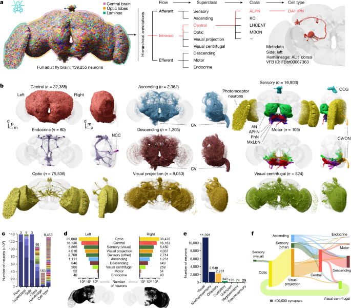
Biological annotation and cell type in the central brain: I. Flow, superclasses, and cell-types with an application to Drosophila
There are multiple categories of central brain associated cells: visual, sensory, and ascending.
Adherents are flow, superclass, class, and cell type. An initial semi-automated approach was used to assign the flow and superclass. See Supplementary Table 3 for definitions and the sections below for details on certain superclasses.
Whether a neuron represents a biological outlier or exhibits sample preparation/segmentation artefacts is recorded in the status column of our annotations as ‘outlier_bio’ and ‘outlier_seg’, respectively. Note that these annotations are probably less comprehensive for the optic lobes than for the central brain. Examples plus quantification are presented in Extended Data Fig. 5.
(2) Some neurons are missing large arbours (for example, a whole axon or dendrite) because a main neurite suddenly ends and cannot be traced any further. This typically happens in commissures where many neurites co-fasculate to cross the brain’s midline. In some but not all cases, we were able to bridge those gaps and find the missing branch through left–right matching. Where neurons remained incomplete, we marked them as outliers.
Source: Whole-brain annotation and multi-connectome cell typing of Drosophila
Enhanced Box Plots for Small Samples, Part I: Annotation and T-Tests for Normally Distributed Samples
Enhanced box plots—also called letter-value plots125—in Fig. 5h and Extended Data Fig. 7f are a variation of box plots better suited to represent large samples. They replace the whiskers with a variable number of letter values where the number of letters is based on the uncertainty associated with each estimate, and therefore on the number of observations. The ‘fattest’ letters are the (approximate) 25th and 75th quantiles, respectively, the second fattest letters the (approximate) 12.5th and 87.5th quantiles and so on. Note that the width of the letters is not related to the underlying data.
After generating the groups, we cross-checked these annotations against current hemibrain and flywire types. In a small number of cases, one hemibrain/cell type was annotated with multiple groups. This occasionally reflected errors in assigning types, which were corrected; and others where individual neurons from a type were singled out due to additional branches/reconstruction issues. We manually adjusted the group annotations to correspond with the hemibrain annotations.
Unless otherwise stated, statistical analyses (such as Pearson R or cosine distance) were performed using the implementations in the scipy123 Python package. T-tests for normally distributed samples were used in order to determine statistical significance.
All of the neuron’s inputs are kept at a constant K. It is definitely a simplification that can be corrected by introducing a distribution P(K) but this requires further detailed modelling.
The global inhibition provided by APL to all of the mixing layer neurons is assumed to take a single value for all neurons. If there were APL and mixing layer neurones, the level of inhibition would be different.
Digital Mirroring of FlyWire and GAL4 Data. I. Identifying all the cell types in the brain from FAFB and reconstruction through the neck
From Fig. 5k, the theoretical values of K that maximize dim(h) in this simple model demonstrate the consistent shift towards lower values of K found in the FlyWire left and FlyWire right datasets when compared with the hemibrain.
For consistency with visualizations and datasets obeying the standard convention (fly’s right on viewer’s left), FlyWire data can be mirrored. To facilitate this, we provide tools to digitally mirror FAFB-FlyWire data using the Python flybrains (https://github.com/navis-org/navis-flybrains) or natverse nat.jrcbrains (https://github.com/natverse/nat.jrcbrains) packages (Extended Data Fig. Through 1c.
The reconstruction was made use of the FAFB dataset 9. A number of consortium members (A. Bates, P. Kandimalla and S. Noselli) alerted us that the FAFB imagery seemed to be left–right inverted based on the cell types innervating the asymmetric body123. A left–right inversion was confirmed after some time. All side annotations in figures, in Codex and elsewhere are based on the true biological side. For technical reasons, we were unable to invert the underlying FAFB image data and therefore continue to show images and reconstructions in the same orientation as in Zheng et al.9, although we now know that in such frontal views the fly’s left is on the viewer’s left. For full details of this issue including approaches to display FAFB and other brain data with the correct chirality, please see the companion paper12.
In order to identify all the cells in the brain, we cross-sectioned all the profiles in the GNG through the neck. We identified all the DNs based on their location in the brain and the main axon branch leaving the brain.
There are two criteria to determine whether or not you can identify ANs: 1) no soma in the brain and 2) a main branch entering through the neck connective.
To identify the words in the ref. 107 in the EM dataset, we transformed the volume renderings of DN GAL4 lines into FlyWire space. Displaying EM and LM neurons in the same space enabled accurate matching of closely morphologically related neurons. For DNs without available volume renderings, we identified candidate EM matches by eye, transformed them into JRC2018U space and overlaid them onto the GAL4 or Split GAL4 line stacks (named in ref. 107 for that type) in FIJI for verification. Using these methods, we discovered all but two cell types in FAFB/FlyWire and annotated them with their published names. A systematic cell type which included their soma location, an e for Em type and a three digit number was given to all the other outstanding DNs. There is an account and analysis of DNs published separately.
Besides the canonical root point, the soma position was recorded for all neurons with a cell body. If the cell body Fibre was truncated or no soma could be identified in the dataset, then this was either based on the entries in the nucleus segmentation table or on selecting a location. These soma locations were critical for a number of analyses and also allowed a consistent side to be defined for each neuron. This was initialized by mapping all soma positions to the symmetric JRC2018F template and then using a cutting plane at the midline perpendicular to the mediolateral (x) axis to define left and right. All the soma positions within 20 m of the midline plane were manually reviewed. The goal was to define a logical side based on examining cell body fibre tracts entering the brain, so that if one neuron was identified as the left and the right it would be annotated. In a small number of cases, for example, for the bilaterally symmetric octopaminergic ventral unpaired medial neurons, we assigned side as ‘central’.
Side refers to whether sensory neurons enter the brain through the left or right nerve. In a small number of cases we could not unambiguously identify the nerve entry side and assigned side as ‘na’.
The central brain has a small number of neurons that can’t be assigned to a specific lineage. These include the primary neurons. The primary and secondary neuralgia form small tracts with which they connect. In the adult brain, morphological criteria that unambiguously differentiate between primary and secondary neurons have not yet been established. It can be found that in cases of experimental proof, primary neurons possess larger cell bodies and cell body fibres. Loosely taking these criteria into account we surmise that a fraction of primary neurons forms part of the HATs defined as described above. However, aside from the HATs, we see multiple small bundles, typically close to but not contiguous with the HATs, which we assume to consist of primary neurons. These small bundles contained 3,780 neurons which were categorized as primary or spurious primary neurons.
Visual sensory neurons (R1–6, R7–8 and ocellar photoreceptor neurons) were identified by manually screening neurons with pre-synapse in either the lamina, the medulla and/or the ocellar ganglia93.
Johnston’s organ neurons in the right hemisphere were characterized based on innervation of the major AMMC zones (A, B, C, D, E and F), but not further classified into subzone innervation as shown previously104. The left hemisphere’s sensory cells were matched to the right hemispheres through the use of the non-biologic method of matching their mirrored morphology. The antennal lobes have thermo sensory and hygro sensory nerve cells that are connected to the uniglomerular projection neurons.
The researchers were able to create a computer model of the fruit-fly brain using the connectome. They tested it by using activated neurons that sense both sweet and bitter tastes. In the virtual fly’s brain, these signals were received by motor neurones associated with the fly’s proboscis. When the sweet circuit was activated, a signal for extending the proboscis was transmitted, as if the insect was preparing to feed; when the bitter circuit was activated, this signal was inhibited. To validate these findings, the team activated the same neurons in a real fruit fly. The simulation was more accurate at predicting the behavior of the fly than it was at predicting the structure of the brain.
New provisional cell types for VPNs and VCNs: ItoLee hemilineage tracts and the Hardenstein nomenclature
98% of the VPNs and VCNs were assigned to specific types. 29 VPNs and 9 VCNs were left untyped, because they could not be confidently assigned a cell type.
There was a double checked hemibrain type split across multiple clusters which led to a split of the hemibrain type.
For VCNs, the nomenclature follows the format [c][neuropil][XX], where c denotes centrifugal; neuropil refers to regions innervated by VCN axons; and XX represents a zero padded two digit number.
To assign cell types to the remaining neurons and in some cases also to refine existing hemibrain types, we ran a double-hemisphere (FlyWire left–right) co-clustering. For VCNs, this was done as part of the per-hemilineage morphology-connectivity clustering described in the ‘Defining new provisional cell types’ section above. We looked at and created a separate clustering on all of the VPNs for which the dendrites are used. Groups extracted from this clustering were also cross-referenced with new literature from parallel typing efforts100,101 and those new cell type names were preferred for the convenience of the research community. In cases in which literature references could not be found, systematic names were generated de novo using the schemata below.
By comprehensively inspecting the hemilineage tracts originally in CATMAID and then in FlyWire, we can now reconcile previous reports. New to the refs. 33,34 (ItoLee nomenclature) are: CREl1/DALv3, LHp3/CP5, DILP/DILP, LALa1/BAlp2, SMPpm1/DPMm2 and VLPl5/BLVa3_or_4—we gave these neurons lineage names according to the naming scheme in refs. 33,34. New to ref. 31 (Hartenstein nomenclature) are: SLPal5/BLAd5, SLPav3/BLVa2a, LHl3/BLVa2b, SLPpl3/BLVa2c, PBp1/CM6, SLPpl2/CP6, SMPpd2/DPLc6, PSp1/DPMl2 and LHp3/CP5—we named these units according to the Hartenstein nomenclature naming scheme. We did not take the following clones from ref. 33 into account for the total count of lineages/hemilineages, because they originate in the optic lobe and their neuroblast of origin has not been clearly demonstrated in the larva: VPNd2, VPNd3, VPNd4, VPNp2, VPNp3, VPNp4, VPNv1, VPNv2 and VPNv3.
There are also 3 types of lineages, VLPl2/BLAv2, and VLPp&l1, with more than two tracts in the clone. Without taking type I and type II tracts into account, we identified 141 hemilineages.
Clustering of Multiple Types in the CoconatFly Package – III: On the Dimensionality of Responses of Multiple K-Clusters
The interface for carrying out such clustering that is implemented in the coconatfly package is streamlined. For example the following command can be used to see if the types given to a selection of neurons in the Lateral Accessory Lobe (LAL) are robust:
There is an optional interactive mode in the web browser. For further details and examples, see https://natverse.org/coconatfly/.
In rare cases, clusters contained a mix of two or more hemibrain types; these were double checked and the hemibrain types corrected (for example, by merging two or more hemibrain types, or by removing hemibrain type labels).
and how it changes with respect to K, the number of input connections. In other words, what are the numbers of input connections K onto individual KCs that maximize the dimensionality of their responses, h, given M KCs, N ALPNs and a global inhibition α?
There are more detailed calculations found in a previous report. Randomized and homogeneous weights were used to populate ({\bf{W}}), such that each row in ({\bf{W}}) has K elements that are 1 − α and N − K elements that are −α. The parameter α represents a homogeneous inhibition corresponding to the biological, global inhibition by APL. The value inhibition is set to be A/M where A is the number ofKCs in each of the three datasets. The primary quantity of interest is the dimension of the KC activities defined by122:
The early rounds of Correct Proofreading Using Ultrastructures: A dataset of 200 cells from the CAVE experiment in a neuronal wiring diagram
The professional team of writers got additional training. Some of the 2D and 3D visual cues used for Correct Proofreading are shown. When false merger or false split result in 3D morphology, proofreaders are unaware of which types of cells they are. Ultrastructures provide valuable 2D cues and serve as good guides for accurate tracing when studied by Proofreaders. Each of them practiced on an average of 200 cells before they were admitted to Production. In this dataset, we determined the accuracy of test cells by comparing them to ground-truth reconstructions. To improve proofreading quality, peer learning was highly encouraged.
Predicting the total time that was required to create the flywire resource is difficult because of the distributed nature of the community, the interlacing of analysis and the variability in how proofreading is done. The second public release, version 783, required 3,013,513 edits. We measured the times when the whole brain was checked during the early rounds. We collected timings and number of edits for 29,135 independent proofreading tasks after removing outliers with more than 500 edits. We were able to work out the average amount of time per edit. However, we observed that proofreading times per edit were much higher for proofreading tasks that required few edits (<5). Our measurements weren’t representative of the second round of correction which went over all segments with more than 100 synapses. These usually required 1–5 edits. We narrowed the calculation to the subset of timed tasks that took the most time, and then we adjusted for that. In round 2, the average time of tasks with 1–5 edits is shown. We averaged these times for an overall proofreading time because the number of tasks in each category were similar. An estimate of 33.1% person-years can be found in the result of an average time of 78 s per edit.
CAVE50 is used to host the proofreadable segment and all of its annotations. CAVE’s proofreading system is the PyChunkedGraph which has been described in detail elsewhere8,124.
Assignment of Central Nervous System Neurons based on Presynaptic Location and Volume using a Collapsyde Method
We assigned synapses to neuropils based on their presynaptic location. We used a method known as ncollpyde to determine the location and assign it to the right place. The rough outlines of the underlying data made some synapses unassigned after this step. We assigned all remaining tassles to closest neuropil if the tass was within 10 m. The remaining sphinxes weren’t assigned.
We used the mesh to calculate the volume for each neuropil. In the aggregated volumes presented in the paper we assigned the lamina, medulla, accessory medulla, lobula and lobula plate to the optic lobe. The ocellar ganglion was assigned to the central brain.
“,,,”fracrmTPrmTP+rmFP R
neuprint had the latest completion rates and numbers for hemibrain. In some cases, neuropil comparisons were not directly possible because of redefined regions in the hemibrain dataset. These regions were not included in the comparison.
The brain of C. elegans stretches from the ring structure to the excretory pores. The authors who called this region the nerve ring include both the anterior portion of the nerve cord and the combined structure as the nerve ring. Nine neurons (RIR, RIV, RMDD, RMD and RMDV) are intrinsic to the nerve ring itself. An additional 26 neurons (AIA, AIB, AIM, AIN, AIY, AIZ, RIA, RIB, RIC, RIH, RIM, RIS, RMF and RMH) are intrinsic to the combined structure, for a total of 35 intrinsic neurons in the brain.
The estimate has error bars due to definitional ambiguities. Ten motor neurons (RMH, RMF and RMD) could arguably be removed from the list, as it is unclear whether motor neurons qualify as intrinsic neurons. The brain could be enlarged by moving the anterior border further away from the excretory pore, which would add 10 neurons. To make these ambiguities explicit, we estimate 35 ± 10 intrinsic neurons. 180 of the 302 central nervous system neurons are involved in the development of the brain. Roughly 15-20% of the brain and 80-90% of the central nervous system are neurones in the brain that are strontium to the brain.
We used CAVEs L2Cache50 to determine cell volumes and surface areas. Volumes were computed by counting all voxels within a cell segment and multiplying the count by the voxel resolution. The area calculation was more complex because it was done through overlap through voxel space. We shifted the binarized segment in each dimension individually and extracted the overlap of false and true voxels. We took the voxels and subtracted the voxel resolution from the dimensions. We added up the estimates for each area. smoothed measured are too compute intensive and will overestimate area slightly.
The Buhmann et al. team trained on the ground truth from the CREMI challenge. The three CREMI datasets contain three 5 × 5 × 5 µm cubes from the calyx in FAFB14 with 1,965 synapses. They evaluated the performance of the classifier on multiple areas, while only using the dataset from Buhmann et al. The performance varies by region.
Eckstein et al.10 created a machine learning model to predict neurotransmitter identities for all synapses from Buhmann et al. based on the electron microscopy imagery alone. Each neurotransmitter was assigned a probability, and each link was assigned a probability for it. They built a database with 3,025 neurons with known transmitters assuming Dale’s law applies. Eckstein et al. reported a per-synapse accuracy of 87% and a per neuron (majority vote) accuracy of 94%.
Each neuron had a Fraction of Presynapses in the right and left hemisphere. The hemisphere was named after it’s opposite side. We excluded neurons that had either most of their presynapses or most of their postsynapses in the centre region.
In order to calculate the rank for each neuron, we used the information flow program implemented by Schlegel and his team. The graph of the sphinx is probabilistically traverses the algorithm. With a certain percentage of the allottedsynaptic area, the likelihood of a neuron being added to the traversed set increased linearly. We repeated the rank calculation for all sets of afferent neurons as seed as well as the whole set of sensory neurons. The group that we used are olfactory sensory cells, the gustatory receptor neuron, and the head and neck bristle mechanosensory cells.
Additionally, we created input seeds by combining all listed modalities, all sensory modalities, and all listed modalities with visual sensory groups excluded.
We ran 10,000 runs for each modality. To assign the percentiles to the neuron according to their rank, we first ordered them according to their rank. For calculating a reduced dimensionality, we used UMAP129 with the following parameters: n_components2, min_dist, and metric: “cosine”.
The Flywire Project: Finding New Neurons and Identifying Their Roles in the Study of COVID-19 and Other Metabolic Diseases
The wiring diagram needed to be checked for errors and the tools aren’t perfect. The scientists spent a great deal of time manually proofreading the data — so much time that they invited volunteers to help. The volunteers and the Consortium members made over 3 million manual edits according to co-author Gregory Jefferis. (He notes that much of this work took place in 2020, when fly researchers were at loose ends and working from home during the COVID-19 pandemic.)
The team was surprised by how the various cells communicate. Hearing and touch, as well as the visual pathway, were important in receiving signals from the single sensory wiring circuit. “It’s astounding how interconnected the brain is,” Murthy says.
The map still had to be annotated, in which the researchers and volunteers labelled each neuron as a particular cell type. Humans would have to verify the results of the software they are trained to use if they wanted to use it on lakes or roads in satellite images. The researchers identified more types of neuron than they had expected. Of these, 4,581 were newly discovered, which will create new research directions, Seung says. “Every one of those cell types is a question,” he adds.
The data about the map1 was published in a package of nine papers. Its creators are part of a consortium known as FlyWire, co-led by neuroscientists Mala Murthy and Sebastian Seung at Princeton University in New Jersey.
Clay Reid, a neuroscience specialist at the Allen Institute for Brain Science in Seattle, Washington, who was not involved in the project but has worked with one of the team members, says it is a huge deal. The world has been waiting for something for a long time.