Probing Climate Change with Bell-Shaped Models: The Effect of Pre-industrial Levels and NNCE in REN_NZCO2

The United Nations has a convention on Climate Change. The Paris Agreement was adopted. The president’s proposal for the UNFCCC, 2015 is available at www.go.nature.com.

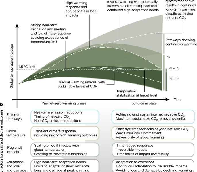
The authors also find that the risk of crossing climate tipping points increases as successive increments above 1.5 °C are reached. The higher the overshoot, the greater the risk of irreversible events -— such as total collapse of the Greenland ice sheet or dieback of the Amazon rainforest — even if carbon-removal technologies successfully bring the warming back to within 1.5 °C.

We need to take a different approach for estimating the second metric (eTCREdown) because the PROVIDE REN_NZCO2 does not have NNCE by design. The scenario was changed with different floor levels of NNCE ranging from 5 Gt CO2 yr1 to 25 Gt CO2 yr1. The scenario is unchanged before 2060. We then calculate the warming outcomes for each of these scenarios applying the same probabilistic FaIR setup and identify the scenario (in this case, REN_NZCO2 with 20 Gt CO2 yr−1 net removals) for which all ensemble members are cooling between 2060 and 2100 (Extended Data Fig. 1). This is required to get an appropriate measure of the effect of NNCE emissions. From this adapted scenario, we evaluate the eTCREdown for each ensemble member using

The bell-shaped ZEC experiments from the ZECMIP modelling protocol are used to diagnose the ZEC for each ensemble member. The experiments use a bell-shaped emissions profile and apply a cumulative emissions constraint from the beginning of the simulation period to the end. The forcers are fixed at pre-industrial levels. The ZEC50 estimate is calculated as the difference between the simulations’ temperatures in years 150 and 100. This ZEC50 estimate is purely used for diagnostic purposes and differs from our eZEC estimate, with the latter dependent on the specific characteristics of the emission pathway we apply. However, as the bell experiments approach zero emissions gradually from above and are similar to the actual mitigation scenario emissions profiles, they are good analogues for eZEC.

Climate feedback is a factor in determining the effectiveradiative forcing from doubling of CO2 and. The parameters F2 and can be used together in FaIR to calculate the ECS for each member of the ensemble.

t2060(n) 1.5quad rmelse.

There is a level of peak warming that depends on eTCREup. We calculate the cumulative NNCE to ensure that post-peak cooling to 1.5 C is maintained.

The metric captures the expected warming until net-zero CO2 is reached and is called the eTCREup.

In our illustrative analysis, we assess the NNCE for the PROVIDE REN_NZCO2 scenario51. The REN_NZCO2 scenario follows the emission trajectory of the Illustrative Mitigation Pathway (IMP) REN from the AR6 of IPCC52,53,54 until the year of net-zero CO2 (2060 for this scenario). The emissions of both GHGs and aerosol precursors remain the same after the year of net-zero CO2.

where ({E}{{{\rm{CO}}}{2},2300}) and ({E}{{{\rm{CO}}}{2},{\rm{pre}}}) are CO2 emission rates from permafrost and northern peatlands in 2300 and in the pre-industrial era, respectively; ({E}{{{\rm{CO}}}{2} \mbox{-} {\rm{we }},2300}) and ({E}{{{\rm{CO}}}{2} \mbox{-} {\rm{we }},{\rm{pre}}}) are CO2-we* due to permafrost and northern peatland CH4 emissions in 2300 and in the pre-industrial era, respectively. The median value of 0.45 C per 1,000 Gt CO2 is used for TCRE.

The Effect of Land Cover Changes on Climate in European Selected CDR Scenarios: a Comparison between piControl and Land-Based Methods

$${E}{{{\rm{CO}}}{2}\text{-}{\mathrm{we}}^{* }}={{\rm{GWP}}}{H}\times \left(r\times \frac{{\Delta E}{{{\rm{CH}}}_{4}}}{\Delta t}\times The times E_rmCH_4right)

When comparing period averages between two scenarios (Fig. 3) or at different times in the same scenario (Extended Data Figs. 6–8), we compare the magnitude of the difference with random period differences of the same length in piControl simulations. If the difference is above the 95th percentile and below the 5th percentile, we consider it to be significant outside of internal climate variability. When n runs are available for the comparison of period averages, we select sets of 2n random periods and compute the difference between the first half and the second half of these random sets to mimic ensemble differences.

The projections for the ss5-34-os and ss 1-19 scenarios are done by 12 ESMs.

The average for land and ocean areas is computed by us after the IA6 regions. WNEU corresponds to land grid cells in western central Europe (WCE) and northern Europe (NEU). The ocean grid cells are above 45 N in the North Atlantic region. 3e,f Land regions are AMZ and WAF.

We note that land cover changes beyond the reference pathway are not included in the two protocols. This points to an implicit assumption that the additional CDR in these simulations is achieved using technical options with little to no land footprint such as Direct Air Capture with CCS (Extended Data Table 2). If the amount of CDR was to be achieved using land-based CDR methods, however, we would expect pronounced biophysical climate effects from the land cover changes alone65. The differences in climate between different regions should be looked at in future modelling efforts.

Governments and industry must focus on how to minimize risks in the future. This means nothing less than aggressively cutting emissions and helping communities to become resilient to the impending shocks. To wait and scrub the atmosphere later is to court disaster — for people and the planet.

It’s not that carbon-removal methods don’t work. Some do. It’s the simplest thing to do, planting trees. More complex measures include removing carbon from the atmosphere. But as Schleussner and his colleagues estimate, up to 400 gigatonnes of carbon would need to be removed from the atmosphere by 2100 to limit warming to 1.5 °C, assuming current emissions trajectories continue. In emissions terms, that is equivalent to running the US energy industry in reverse for around 80 years.