Derivation of global mean SST trends in 1871-1910 and 1901-1940 using a method of emergent constraints44. Application to large-scale climate models

There are constraints on SST trends. We derived emergent constraints on global mean SST trends in the period 1871–1910 (ocean cooling) and for the early-twentieth-century-warming period (1901–1940). The CoastalHybridSST dataset7 and HadSST4 were used to deriveConstraints. We related all datasets to global mean SST trends using an emergent constraint technique44 explained in the next paragraph.

In Fig. 5, we constrained the ranges of global mean SST trends in the 1871–1910 and 1901–1940 periods using the different observation-based datasets (longer periods, 1871–1920 and 1901–1950, are shown additionally in Supplementary Fig. 8). To derive those uncertainty ranges, we applied the method of emergent constraints44, which uses the relationship between an observable metric (predictor metric) and a target metric across an ensemble of climate model simulations to constrain the target metric based on the observable climate metric. In our application, the predictor metrics and the target metric consisted of temperature trends from the same time period but for different large-scale regions. The GMSST trend in the periods 1871– 1910 and 1901–1940 were the targets. Predicted GMSST trends for the HadSST4 and CoastalSST datasets were predictions of the predictor metrics. We first verified that CMIP6 historical simulations (including individual ensemble members to capture internal variability) show a strong linear relationship between our target metric and the respective predictor metrics. We found correlations with the temperature trends of the Pearson correlations. The linearity between land and ocean warming is expected from physical theory43. We used least squares linear regression to derive prediction intervals for our target metric. Forty-four. Linear regression between two univariate variables y and x is given by y = β1x + β0 + ϵ, where β1 is the regression slope and β0 is the intercept. Least-squares linear regression minimizes the least-squares error

Comparing the ocean and land temperature reconstruction in the CMIP6 models based on observational data and palaeoclimate proxy records

There are a number of samples available. There is an estimate of the slope of the regression. The ‘prediction error’ of linear regression is given by44:

The temperature difference of the ocean and land. We compared the difference between the ocean and land-based reconstructions for a given metric. The observationally derived (\Delta {\widehat{{\bf{T}}}}{{\rm{O}}\text{-}{\rm{L}}}^{{\rm{GMST}}}), including the error realizations, was compared with the equivalently masked reconstruction range of ocean and land temperatures in the CMIP6 models ((\Delta {\widehat{{\bf{T}}}}{{\rm{O}}\text{-}{\rm{L}},{\rm{CMIP}}6}^{{\rm{GMST}}})), and shown in Fig. 2 along with a low-pass and a high-pass filtered version.

Second, we analysed a regional SST reconstruction33, which is based on only ocean proxy records. The ocean proxy records are derived exclusively from annually or seasonally resolved tropical coral archives. Temperature estimation is based mainly on oxygen isotopic composition (δ18O of coral carbonate), but records based on the skeletal Sr/Ca ratio and coral growth rate are also included. Reconstruction targets are regionally averaged tropical SST anomalies at the annual timescale for four large-scale ocean basins: the western Atlantic, the eastern Pacific, the western Pacific and the Indian Ocean. The study uses a weighted CPS approach, using a nesting procedure to address the changing number of available observations over time. The proxies are weighted. The magnitude and significance of the variance of each record’s contribution to the total is weighed against its relationship with SST anomalies. Depends on different weighting schemes and calibration periods are accounts by an ensemble of reconstructions. The best reconstruction is chosen based on the lowest cumulative error score over the validation period. We analysed individual palaeoclimate proxies.

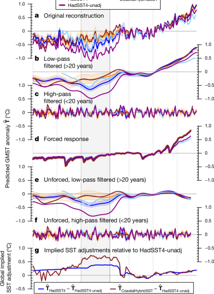
The GMST reconstructions are analysed by applying timescale filters and an Attribution method. The low pass Butterworth filter is used for a period of 20 years to separate our original reconstruction from the low pass and high pass filters.

The focus of the paper is to understand and compare the global temperature reconstructions obtained independently from the Had SST4 dataset and the CRUTEM5 LSAT dataset, which are both subject to varying incomplete coverage and affected by time-evolving uncertainties and biases. Both datasets have been developed and maintained over decades and they are important to the Intergovernmental Panel on Climate Change process. We wanted to compare the SST, LSAT and night-time marine air temperature datasets with our reconstructions on a like by like basis, so we created a land-based reconstruction using an alternative LSAT dataset. The models were trained with CRUTEM5 coverage and a few missing grid cells were filled using nearest-neighbour. Berkeley Earth Land is based on the Global Historical Climatology Network MonthlyTemperature Dataset55, Version 4, with a higher number of weather stations than the newer CRUTEM5 and compared favorably to a recently altered land dataset18. We projected all three datasets onto the coefficients obtained from the CMIP6 SSTs that were masked to HadSST4 coverage. The coverage of COBE-SST2 and ERSST5 is larger than HadSST4 but there are a few missing grid cells.

Once regression coefficients were extracted following the methodology described above, we obtained observation-based predictions for all target metrics by using the spatially incomplete CRUTEM5 and HadSST4 data as inputs to the regression models (equations (4) and (5)). The comparison of our observation-based reconstruction with CMIP6 models in Fig. 2 was based on 602 CMIP6 historical simulations that contain ‘tas’ and ‘tos’ data, that is, 98.835 model-years (overview in Supplementary Table 4), which were masked and reconstructed with observational coverage for each time step.

Three historical ensemble members from each model were selected for the training of the regression models. The training dataset consisted in total of 15,626 model-years, and an overview of the CMIP6 models used for training is given in Supplementary Table 4. When it came to training the regression models for each m, they only used the monthly data from the same month in CMIP6 models.

For the gridded fields as regression predictors, we extracted the variables ‘tas’ (near-surface air temperature) and ‘tos’ (sea surface temperature) from climate model historical (1850–2014) and 2014–2020 simulations following the Shared Socioeconomic Pathway (SSP) 2-4.5 scenario that contributed to the CMIP6 multi-model archive50. The simulations were refashioned to a grid that was the same as the CRUTEM 5 and HadSST4 grids. All climate model data were centred based on a 1961–1990 reference period, in accordance with CRUTEM5 and HadSST4 data processing.

The regression coefficients were obtained by using a standard cross-validation approach. Cross-validation is a common practice in data science, dividing the raw dataset into different, distinct folds. This ensures that model fitting and validation occur on distinct data subsets, preventing biased performance evaluations. The method of cross-validation used in climate science uses a strategy called leave one model out, similar to an iterative perfect model approach. In this process, for a total of k CMIP6 models, the ridge regression model is iteratively fitted on k − 1 models and validated on the kth model (referred to as ‘leave-one-model-out cross-validation’). This iterative approach guarantees that the regression coefficients generalize effectively to an unseen model, ensuring the robustness of the statistical model across the CMIP6 multi-model archive. The tuning parameter λ is then selected during cross-validation to minimize the mean squared error on out-of-fold data, and the corresponding regression coefficients are extracted. The final set of regression coefficients is obtained as the average across the k model fits. Each climate model gets the same amount of weight for the regression coefficients as the number of ensemble members.

This results in a small but non-zero regression coefficients. The tuning variable determines the extent of shrinkage and is determined via cross- validation, as mentioned in the following paragraph. The intercept of the linear model is not shrinked.

mathoprmarrmgrmmrmirmnlimits

There is a linear regression problem with a high dimensionality, where there can be considerable predictors of p. Ordinary least squares aim to reduce the residual sum of squares. However, in high-dimensional settings, regression coefficients lack proper constraints, so relying on this single objective may be problematic. Ridge regression is a method that can be used to address collinearity issues. Ridge regression prevents overfitting by incorporating a penalty for model complexity through the shrinkage of regression coefficients. The shrinkage is based on the sum of squared regression coefficients (referred to as L2 regularization) and a ridge regression parameter λ that governs the degree of shrinkage. Consequently, ridge regression addresses a joint minimization problem expressed as

Source: Early-twentieth-century cold bias in ocean surface temperature observations

HadCRUTEM5: The HadSST4 Ensemble of Uncertainties in Near-surface Air Temperature and LSAT Anomalies

$$\begin{array}{l}{X}{{\rm{m}}{\rm{o}}{\rm{d}},{\rm{O}}{\rm{c}}{\rm{e}}{\rm{a}}{\rm{n}}:1895\text{-}06}^{\ast }={X}{{\rm{m}}{\rm{o}}{\rm{d}},{\rm{L}}{\rm{a}}{\rm{n}}{\rm{d}}:1895\text{-}06}+{{\boldsymbol{\epsilon }}}{{\rm{b}},{\rm{O}}{\rm{c}}{\rm{e}}{\rm{a}}{\rm{n}}:1895\text{-}06}\ \,\,\,+\,{{\boldsymbol{\epsilon }}}{{\rm{p}},{\rm{O}}{\rm{c}}{\rm{e}}{\rm{a}}{\rm{n}}:1895\text{-}06}+{{\boldsymbol{\epsilon }}}_{{\rm{u}},{\rm{O}}{\rm{c}}{\rm{e}}{\rm{a}}{\rm{n}}:1895\text{-}06}.\end{array}$$

Following the method given in ref, uncertainties are found in CRUTEM5. The name of the store is 52. A 200-member ensemble of potential realizations of known, temporally and spatially correlated uncertainties in near-surface air temperature has been produced as part of the HadCRUT5 Noninfilled Data Set13 (that is, ϵb,Land(s, t)). The corresponding ensemble of CRUTEM5 LSAT anomalies has been extracted from this, using the HadSST4 ensemble to unblend SST and LSAT anomalies in coastal grid cells. The ensemble realization of biases encompasses uncertainties such as station-based homogenization errors and uncertainty in climatological normals, as well as regional urbanization errors and non-standard sensor enclosures (full description provided in refs. 13,22,52. In the form of gridded error fields, uncorrelated uncertainties are available.

$${{\bf{Y}}}{{\rm{mod}}}^{{\rm{GMST}}}={X}{{\rm{mod}},{\rm{Ocean}}:1895\text{-}06}\,{\widehat{{\boldsymbol{\beta }}}}_{{\rm{Ocean}}:1895\text{-}06}^{{\rm{GMST}}}+{\boldsymbol{\epsilon }}.$$

After estimating the regression coefficients, we predicted each target metric at each time step based on SST or LSAT observational datasets, and the actual coverage. For example, for June 1895, LSAT and SST predictions of GMST would read as

It is known as the “X_rmmod” or “rmLand” and it is also called the “boldsymbol”.