Obtaining accessibility for the fetal and adult K562 chromatin accessibility atlas from multiome data augmented with a GET model
The fetal and adult chromatin accessibility atlas was first published by Domcke et al.1, and we have used the peak set produced by Zhang et al.2 to incorporate it. The fetal only GET model was trained with the same peak calling and cell type annotations as the Domcke et al.1 model. For the 10× multiome data, we used the provided peak fragment count matrix. For the K562 NEAT-seq and bulk chromatin accessibility data, a more permissive version of peaks was called using MACS2 (ref. 60), and different logCPM cutoffs were applied to the resulting peak set to select accessible regions. The data augmentation improves the diversity of inputs and the model for data from a single cell type.
We collected the sequence element library and created a vector sequence for inclusion with the help of the Get program. We then followed the same data preprocessing procedure to get the motif scores of the inserted elements. We performed in silicoinserting, by summing the score with an existing region on the genome. The ±100 regions centred around the insertion region were then used as an input sample for GET to make expression predictions. The mean predicted expression was compared to the predicted accessibility as a prediction of regulatory activity. For each region, we performed 600 insertions across the genome to match the experimental insertion count. We used the GET model to perform the inference. In total, in silico lentiMPRA of all 200,000 elements in K562 took around 5 days.
We stratified the K562 lentiMPRA elements (approximately 200,000) by overlapping the annotated 15 ENCODE ChromHMM states computed from histone mark and other ChIP–seq data for K562. The elements with the same state as 12 EnhBiv were enhancers and those with a state similar to 13 ReprPC were repressive.
Multiple input-format dependent Jacobian analysis with ATAC models using g:Profiler for gene enrichment analysis at a large number of genes
The Jacobians use a matrix to evaluate the change in output dimensions when each input format is used. It’s important that we pick the strand and output dimension that correspond to the given gene.
The feature (motif) importance vector ({{\rm{v}}}_{g}\in {{\mathbb{R}}}^{m}) is obtained by multiplying the gradient element-wise with the original input and summarizing across regions:
where (\odot ) signifies the element-wise or Hadamard product. When we infer (J_X) using a ATAC model, the (X) is used because it’s the main feature–feature interaction analysis matrix. This facilitates study of the relationship between regulators and observed chromatin accessibility.
The (rmv_g) across the genome is acquired by concatening the cell-type-specific genome-wide gene-by-midtif matrix for cell type c. Different cell types can be applied to the same process.
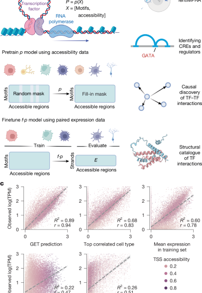
All options were provided to users in our packages and we used multiple features attribution methods in different analyses. When we change a small amount of the input along a dimensions, the model output will go up or down according to the gradient of the model. The generalization to multiple outputs in the context of neural network feature attribution extends to the Jacobian matrix ({J}{i,j}=\frac{\partial {f}{i}}{\partial {x}_{j}}), where fi is the ith output, representing the transcription level on either the positive or negative strand, and xj is the jth input feature, comprising scanned and summarized binding scores for 282 TF motif clusters and an extra dimension for accessibility scores. The Jacobian matrix can be computation to understand the influence of individual features on the levels.
We can use the genes-by-motif matrix to make a choice and then we can look at the biggest entries in the column to figure out which genes will be most affected. The top 1,000 genes were chosen and we used g:Profiler to do gene enrichment analysis. We filtered the results using term size (gene number in a term definition) greater than 500 and less than 1,000. The terms with an adjusted P value less than 0.05 were retained as significant terms. We further selected TFs in the ‘Hemopoiesis’ term with expression log10(TPM > 1) for visualization against the GATA motif score.
This analysis sought to piece together the relationships between the expression of target genes in different cell types. A unified structure comprised of genes, motifs and cell features was developed from the aggregated and organized Gene-by-Modifi files. We identified the target genes for each TF within predefined motif clusters and computed the mean expression levels of both the target genes and the corresponding TFs. Fetal cell types and adult cell types were analysed to avoid artifacts caused by experimental batches, and we found similar results. The analysis was performed iteratively for all TFs within the motif clusters specific to fetal cell types.
We feed the sample into the RegionEmb layer and use it to make a regulatory element with a dimensions of 768 for each peak. As we do not want to lose information in the input of the original regulatory element, we apply a linear layer to capture the general information in the different classes of TF binding sites. To learn the cis- and trans-interactions between regulatory elements and TFs, we apply 12 Encoder layers with a multihead attention (MHA) mechanism on the regulatory element embeddings.
Spearman correlation was performed using the same matrix in both cell type specific and cell type agnostic settings. The matrix was made using input gradient scores. The correlation calculation was used for the cell-type-specific settings because all genes with promoter overlap were used. Causal discovery was performed on the gene-by-motif matrix using LiNGAM69. A random sample of 50,000 genes were randomly plucked from all types of cells and used to make a matrix for the cell type agnostic settings.
We downloaded the known physical interaction sub network from the STRING database and kept interactions with a combined score greater than 400 as the ground truth label. We mapped the physical interactions between these objects on the basis of the motif cluster annotations. The precision of the network was calculated after comparing it with our prediction. We mapped all significant interactions that were determined by mass spectroscopy40 to the different types of interactions. The colocalization results from the tracks of ChIPP– seq in HepG2 are compared to those from the tracks of TF Atlas. The method for calculating colocalization is documented. The peak sets were divided into three tiers (high, mid and low). Then, for a pair of TFs P1 and P2, we checked colocalization between every tier pair and assigned scores with a preference for high–high colocalization (score = 9). If the strong binding peaks of P1 overlapped with strong binding peaks of P2, the P1–P2 interaction was considered to be more robust than in the case in which the P1 strong binding sites only overlapped with the P2 weak binding sites. We show the colocalizations in a stronger manner than mid–mid interactions. These are the more reliable interactions. A stronger cutoff reduced the performance to a 0.097 macro F1 score at 2% recall.
pLDdt from AlphaFold is reliable as it accurately predicted structure. The high and low pLDDT regions were categorized into each sequence. We found that 80% of the known domain can be easily identified by using high pLDDT regions, and a high ratio of positively charged residues. We used a ten-amino-acid moving-average kernels to computed smoothed pLDDT and then we normalized it by dividing by the maximum. After that, any region that had a smoothed pLDDT score less than 0.6 was defined as a low pLDDT region. If two low pLDDT regions were close, they were merged into one. Any region that was not a low pLDDT region was labelled as a high pLDDT region.
The initial configuration was prepared from the AlphaFold predicted PDB file. The force field was used for system parameters. A box size of 1nm was used to define a simulation box. The system was solved using a water model through the solvate module. To neutralize the system and generate physiological ion concentrations, sodium (Na+) and chloride (Cl−) ions were added using the genion module. The energy minimization terminated upon reaching a maximum force below 1,000 kJ mol−1 nm−1. Each minimization iteration used a step size of 0.01 and was configured to run for a maximum of 50,000 steps. The system was then equilibrated in two steps: first in the NVT (constant number, volume, temperature) ensemble and then in the NPT (constant number, pressure, temperature) ensemble for 100 ps of simulation time. A 100 ns production run was then performed, and trajectories and energy profiles were stored for subsequent analysis. All configs of these are available at the Proscope repo (https://github.com/fuxialexander/proscope). In our analysis, we found that the per-residue pLDDT scores for ZFX, IDR and TFAP2A in the multimer structure were correlated strongly with residue instability, as measured by root mean squared distance, consistent with the results of previous studies indicating that AlphaFold implicitly learns protein folding energy functions.
Source: A foundation model of transcription across human cell types
Antibody and chemiluminescence studies of HeLa and REH Cells (CCL-2) and mycoplasma cell lines obtained from ATCC
HeLa cells (CCL-2) and REH cells (CRL-8286) were purchased from ATCC. Cell lines purchased from a certificated cell line bank were not further authenticated. All cell lines were negative for mycoplasma. No commonly misidentified cell lines were used in the study.
HeLa cells were cultured in DMEM (Gibco, catalogue no. 11965) supplemented with 10% defined fetal bovine serum (HyClone, SH30070), at 37 °C and 5% CO2. HeLa cell lysates were made using a lysis buffer of 50% NP-40 and a phosphatase and protease inhibitor cocktail. Samples were incubated with 5 µg agarose-conjugated TFAP2A primary antibody (Santa Cruz Biotechnology, sc-12726 AC) overnight at 4 °C before being run in Laemmli loading buffer (BioRad, 1610737). Proteins were separated on 10% Tris–glycine gels (ThermoFisher, XP00100), transferred to polyvinylidene fluoride membranes (Immobilon-P, IPVH00010) and probed with primary antibodies against TFAP2A (ABclonal, A2294, 1:750), ZFX (ThermoFisher, PA5-34376, 1:500) and β-actin (Santa Cruz Biotechnology, sc-47778, 1:10000), followed by chemiluminescence detection. A repeat experiment was performed for coimmunoprecipitation negative controls, which were probed with primary antibodies against SRF (Abclonal, A16718, 1:750) and β-actin (Cell Signaling Technology, 4967, 1:10000), followed by chemiluminescence detection.
We initially cloned PAX5-WT and the PAX5 G183S mutant into the pCDNA3.1-MCS-13Xlinker-BioID2-HA (Addgene, catalogue no. 80899)71. We subcloned the two units, PAX5-WT-13Xlinker- BioID2HA and PAX5-G183S-13Xlinker-BioID2HA, into the pCDH- GFP-puro vector. We transduced the REH B-ALL cell line (ATCC, CRL-8286) with pCDH-PAX5-WT-13Xlinker-BioID2-HA-GFP and with pCDH-PAX5-G183S-13Xlinker-BioID2-HA-GFP and selected transduced cells with puromycin (1 μg ml−1) to generate stable cell lines. The proximity labelling assay was performed following previously published methods71,72,73. Briefly, the REH stable cell lines had control over pCDH-PAX5-WT-13xlinker-HA-GFP. We collected the cells, washed them twice in cold brine, and then placed them on ice for 50min with a lysis buffer of 150 mM. NaCl, 10 mM KCl, 10 mM Tris-HCl pH 8.0, 1.5 mM The supplemented with the IGEPAL and a small amount of the MgCl, 0.4% IGEPAL, and 63 U of the benzonase. At 4C, the centrifugation resulted in the clearance of the proteins at 20,000g. We performed total protein quantification using a Pierce BCA Protein Assay kit (ThermoFisher Scientific, catalogue no. 23225) and incubated 1 mg of total protein extract with 100 μl of magnetic streptavidin beads (Dynabeads MyOne Streptavidin C1, Life Technologies, catalogue no. 65002) on a rotator at 4 °C overnight to isolate biotinylated proteins. We washed the beads twice with lysis buffer, once with 1 M KCl, once with 0.1 M Na2CO3, once with 2 M urea 10 mM Twice, with the lysis buffer, the Tris-HCL was pH 8.0. A 4protein loading buffer was supplemented with 2 mM biotin, 50 mM dithiothreitol, and a 10 min boil. Standard protocols and the following antibodies were used to detect the presence of a hin ding in total protein extracts or immunoprecipitates. S911, 1:1000), anti-PAX5 (Cell Signaling, catalogue no. 8970, 1:500), anti-HA (Cell Signaling, catalogue no. 3724, 1:1000), anti-NR2C2 (Cell Signaling, catalogue no. 31646, 1:500), anti-NCOR1 (Cell Signaling, catalogue no. 5948, 1:500), NRIP1–HRP (Santa Cruz Biotechnology, sc-518071, 1:200) and NR3C1 (Cell Signaling, catalogue no. 12041, 1:500). A Li-Cor Odyssey OFC instrument and the GelAnalyzer 23.1 software were used for the analysis of the samples.
The experimental procedure involves designing a library of lentivirus vectors that contain both desired sequence elements and a mini promoter. The regulatory activity is measured through the use of a log copy number of transcribedRNAs and integrated DNA copies.
Source: A foundation model of transcription across human cell types
Towards a foundation model of transcription across human cell types: Predicting Cell-Type-Specific 3-Dimensional Contacts with a Two-Layer Convolutional Neural Network
This model could be improved in future work by taking GET region embeddings as further input and learning to predict cell-type-specific three-dimensional contacts.
To make them comparable across genes, each score was normalized across the 100 peaks of the genes.
Recent studies show that one-dimensional genomic distance is the main factor governing the effects of CRISPRi enhancers. Most methods include a component of the genomic distance. Enformer has a form of decay in its encodings. HyenaDNA incorporates a sinusoidal positional encoding over the DNA sequence, and our benchmarking results follow an exponential decay from the TSS (Fig. 3c; NFIX). We have added distance information to the GET. In particular, we designed a simple DistanceContactMap module for GET to convert the pairwise one-dimensional distance map between peaks to a pseudo-Hi-C contact map. DistanceContactMap is a simple three-layer two-dimensional convolutional neural network (kernel size: 3) with ({\log }_{10}(\text{pairwise distance}\,+\,1)) as input and SCALE-normalized observed contact frequency as output. The model was train using a negative log-likelihood loss. The data utilized for training ABC Powerlaw was the same as K562 Hi-C data used for DistanceContactMap, which produced a correlation of 0.855 Pearson. We call it the prediction of the model ‘GET Powerlaw’. The other two scores shown in Fig. 3d are defined as follows:
We use the largest pretrained model available through Hugging Face. To score enhancer–gene pairs, we performed in silico mutagenesis by knocking down the enhancer element (that is, setting each base pair in the enhancer region to the unknown nucleotide N in the vocabulary set) and comparing against the wild-type likelihood of observing the promoter sequence.
Enformer was used with a background normalization procedure described by Gschwind and colleagues.
Source: A foundation model of transcription across human cell types
The ABC Powerlaw in the ATAC model with K562 Hi-C data, adapted with minimal training and limited reference datasets: a study of single tumours
The ABC Powerlaw was computed by adding up the powerlaw function in the official ABC repo with, and scale 594, and the values that had been trained on K562 Hi-C data.
We mainly used the ATAC model in our analysis. This approach offers improved attribution to sequence features, ensuring that the model does not overly depend on accessibility signal strength as a surrogate for sequence characteristics.
We tested the procedure using a single patient sample from a new dataset. We tested the model against a pretrained zero-shot model on 16 held-out patient samples. To ensure a robust evaluation, we did not include two patients in the analysis. A Pearson correlation of more than 0.9 is achieved when fine- tuning a single tumours patient sample, whereas zero-shot performance achieved a 0.67 Pearson correlation. This proves that the model can quickly adapt to new datasets with minimal training. As the availability of multiome data continues to grow, more comprehensive reference peak sets will assist in the adaption of the GET model to a broader range of cell types and experimental conditions.
Cell type purity and heterogeneity: the dynamic and heterogeneous nature of certain cell types, such as stem cells, and the precision of identification and classification of cell types can introduce variability in gene expression profiles, complicating the prediction task.
Cell type rarity and library size: rare cell types often have smaller data libraries, which can limit the model’s learning potential and affect the accuracy of predictions.
Source: A foundation model of transcription across human cell types
SVM fine-tuned Enformer on K562 CAGE and RNA-seq for a leave-out peak set across chromosome 14
SVM: we used scikit-learn Support Vector Regression with epsilon 0.2, linear kernel and max iterations 1,000. Two-dimensional output was handled by MultiOutputRegressor.
For the K562 prediction, we performed leave-one-syndrome prediction for all the autosomes and found an average Pearson correlation of 0.81. For K562 CAGE prediction, we used GET to predict K562 CAGE (FANTOM5 sample ID: CNhs12336). We note that this comparison privileges Enformer, which was trained extensively on CAGE tracks, including K562 (track ID: 4828 and 5111), whereas GET needed to be transferred to the new assay. Here we evaluated fine-tuned GET against Enformer predictions summed across the two CAGE output tracks for a leave-out peak set across chromosome 14. We selected chromosome 14 because it did not appear in the public Enformer checkpoint’s training or validation set. Pretrained GET was fine-tuned in three ways.
QATAC from BATAC pretrain: in this setting, the base model was trained on the fetal–adult atlas with binarized ATAC signal; in the fine-tuning, we used the original aCPM ATAC signal.
The leave-out-astrocyteRNA-seq prediction model was trained on the fetal accessibility and expression atlas to be the base model. We further fine-tuned this model using quantitative ATAC signal.
Source: A foundation model of transcription across human cell types
Transfer of pretrained GET to functional genomics assays: A case study on the bulk ATAC prediction and the K562 CAGE dataset
These experiments leveraged LoRA parameter-efficient fine-tuning to achieve significant gains in time and storage complexity. On a single RTX 3090 GPU, all fine-tuning converged within 30 min, resulting in a 3 MB K562-CAGE-specific adaptor that could be merged into the base model.
Here we show results for transfer of pretrained GET to different functional genomics assays. We collected the data for the bulk ATAC prediction for K562. After calling peaks using MACS2 with default parameters, we computed the log(aCPM) by counting Tn5 insertions located inside the peak and filtered out the peaks with log(aCPM) less than 0.03. For scanning and prediction, peaks and a CPM were used. We performed leave-one-chromosome-out fine-tuning using 200 peaks per input sample. The base checkpoint was trained on the fetal and adult atlas with the binarized ATAC setting and 200 peaks per input sample. LoRA was used for all layers. The model started to over fit after the fine-tuning took around 160 s to complete. For fine tuning, Pearson correlation was collected at a number of epochs. For CAGE prediction, we collected the K562 CAGE (CNhs12336) BAM file from FANTOM5 and used bedtools to extract alignment counts in peaks called from ENCODE K562 scATAC-seq data (ENCFF998SLH). The base model for fine-tuning was used along with the ATAC information and the input sample in three settings.
In general, GET showed robust performance when leaving out one to ten motifs. The performance was degraded when using 20 motifs with a cutoff of 20%, due to the removal of most of the training data.
It is difficult to apply a model that has been trained on just one dataset to a new platform because of the biases. Thus, for a new dataset with multiple cell types available, we took a leave-out cell type approach to fine-tuning. For a dataset of sorted cell types where only one cell type was available, we used leave-out chromosome training.
There is a main challenge in adapting the model to the new data and that is compatibility between the training spaces and the new data. Variations in cell types, sequencing technologies and preprocessing pipelines can result in substantially different ATAC peak sets, potentially leading to incompatible input and embedding spaces. We came up with a plan to create a compatible peak set with new and training peak sets. When overlaps occur between training and new peaks, we assign priority to the training peak set coordinates. Unique peaks from the new data are incorporated as they are. Peak lengths in the fetal–adult atlas have remained consistent despite training and new datasets. The comprehensive coverage of our fetal-only/fetal–adult peak set (1.3 M peaks) typically results in new, unseen peaks contributing less than 10% of the total peaks. This approach has demonstrated promising transferability to various data types, including SHARE-seq data of perturbed human embryonic stem cells and 10× multiome GBM data.
Source: A foundation model of transcription across human cell types
Self-Supervised Training for Regulatory Element Prediction with Low-Rank Adaptation in Masked Autoencoders and Random Forests
The Random forest was used with ten estimators and max depth 10. MultiOutputRegressor was used to handle two-dimensional output.
CNN: three Conv1d layers (layer dimensions: 283 input, 128, 64, 32, 3 kernel size) followed by FC(32, 512) → ReLU → FC(512, 2); SoftPlus was used for output activation. The same parameters, optimizers, and programs were used for GET and we used them.
GET provides an option to perform parameter-efficient fine-tuning over any specific layer through low-rank adaptation (LoRA)64. This is commonly used to adapt to a new assay or platform; we apply LoRA to the region embedding and encoder layers, while doing full fine-tuning on the prediction head. 99% of the parameters were reduced by this.
Early stopping: to optimize performance and prevent overfitting, we used early stopping on the basis of validation loss, enabling us to select the best model checkpoints for subsequent evaluation.
We take the output from each head h and put it into the attention block. The layer normalization (LN), feed-forward network (FFN) and residual connections are finally used to generate the output for each layer. Thus, the mechanism behind the regulatory-element-wise attention block can be summarized as:
Similar to the Vision-Transformer-based Masked Autoencoders62, we replaced the regions in the selected positions with a shared but learnable ([{\rm{MASK}}]) token; the masked input regulatory element is denoted by ({X}^{\text{masked}}=(X,M,[{\rm{MASK}}])), where (X={{{x}{i}}}{i=1}^{n}) is the input sample with (n) regulatory elements. Predicting the original values of the masked elements is the training goal. Specifically, we take masked regulatory element embeddings ({X}^{\text{masked}}) as input to GET, while a simple linear layer is appended as the prediction head. The overall objective of self-supervised training can be formulated.
The PyTorch framework is used for the GET implementation. For the first training stage, we applied AdamW as our optimizer with a weight decay of 0.05 and a batch size of 256. The model was trained for 800 epochs with 40 warmup epochs for linear learning rate scaling. We set the maximum learning rate to 1.5 × 10⁻⁴. The training usually takes around a week for a cluster with 16 V100 GPUs. For the second fine- tuning stage, we used AdamW63 as our optimizer, with a weight decay of 0.04 and a batches size of 256. The model completes in about 8 h using eight A 100 graphics processing units. Screening for all genes in a single cell type takes several minutes, and can be done large-scale.
There is a description of the computation infrastructure and convergence criteria used in the section below.
The fine-tuning was done on eight NVIDIA A100 GPUs, ensuring consistency in computational resources.
The process was done in one day, with 100 epochs. It is important for adapting the pretrained model to specific tasks.
rnz_lprime +{{\rm{z}}}_{l}^{{\prime} },$$
Where w_q,W_kin mathbbR.
Source: A foundation model of transcription across human cell types
Mapping the cell-type-specific accessible regions of Tabula Sapiens 24 using a logarithmic progression function (CPM) procedure
For identification of cell-type-specific accessible regions, the peak calling results from the original studies of each dataset were used to obtain a union set of peaks. Subsequently, to compile a list of accessible regions specific to each cell type, we filtered out peaks with no counts.
The accessibility score for a specificgenomic region was determined by the number of fragments located within it for a given cell type pseudobulk. To enhance the generalizability of the model, these counts were further normalized through the logCPM procedure. Specifically, let t be the total fragment count in a pseudobulk, and let ci be the fragment count in region i. Then, the accessibility score si can be computed as:
For experiments encompassing multiomics, the correspondence between accessibility and expression was inherently determined through cell barcodes. In pseudobulk cases, cell type annotations were used to facilitate the mapping. Fetal celltypes from the fetal expression atlas were used to derive adult data from Tabula Sapiens 24. When several ATAC pseudobulk shared the same cell type annotation, identical expression labels were assigned. This compromise was necessitated by the current dearth of multiome sequencing data, a situation expected to change dramatically in the near future.
To improve training stability, we log-transformed the expression values as log10(TPM + 1). We mapped the gene expression to accessible regions using the following approach, in order to overcome the problem of being at gene level, not transcript level. If a promoter had a CPM less than 0.05), the corresponding expression value was set to 0. Each regulatory element was assigned an expression target value.
In alignment with the 200 × 283 input matrix, the target input is a 200 × 2 matrix, symbolizing the transcription levels of the corresponding 200 regions across both positive and negative strands.