Hydrodynamic Modelling of the Southern North Sea: Input Ice-Sheet Reconstruction and Sea-Level Effects in the Low-Coalescence Regime

We used 1D and 3D models to model drivers in the southern North Sea. All models (1) require an input ice-sheet reconstruction, which defines the spatial and temporal history of major grounded ice sheets during the last glacial period, and (2) solve the generalized sea-level equation by including time-dependent shoreline migration as well as sea-level change in regions of ablating marine-based ice67. The influence of rotation of Earth on the sea-level calculation is only included in the 1D GIA models. However, comparison of the results from the 1D GIA model with and without rotation showed negligible differences across the study period. The Earth model has a main difference between the 1D and 3D models. In the 3D GIA model, the viscosity varies both laterally and with depth, whereas in the 1D GIA model, viscosity varies only with depth.

Fox-Kemper, B. et al. in Climate Change 2021 – The Physical Science Basis: Working Group I Contribution to the Sixth Assessment Report of the Intergovernmental Panel on Climate Change. Cambridge Univ.’s ch 9 Press in 2023.

The 3D GIA model of the Deep North Sea from NAISC 87 and its reconstruction using XRF-scanned vinorkins

National databases helped to find offshore locations with good prospects of preserved flora and fauna. Sub- bottom profilers, boomers and sparkers were used during the research cruises in order to map the distribution and depths of the 4,400 line km of peat. The vibrocores were cut in metres, then split, and then stored for all cruises at a time of the year that is 4 C. The XRF-scanned vinorkins were used for the cruise ships for the next two years.

Contributions from the NAISC were calculated using a recently published reconstruction of its extent through the Holocene8. The Mapped NAIsc areal extents were converted to ice volume using a relationship between dome-shaped ice-sheet sectors. It has been used in some parts of NAISC 87, but not for the rest. The estimates of uncertainty in the ice-sheet were used to calculate the ice-volume uncertainty. The reconstructed ice-sheet volume for the 11 ka period must be the minimum ice-sheet volume and the maximum ice-sheet volume. 8).

The method of ref was used to create a finite-element model for the 3D GIA model. 72 with locally enhanced spatial resolution73. The high-resolution zone is centred on the Southern North Sea and has spatial resolution of around 25 km. The resolution outside this zone is increasing from 50 km to 200 km. Today’s topography was obtained from the same source. The models were constructed with two approaches. The first approach converts the seismology anomalies to the temp anomalies using partial derivatives of the seismic velocity to temperature. The conversion assumes that velocity anomalies are caused by thermal anomalies, although compositional anomalies could also have a role. Therefore, we vary a scale factor between 0 and 1 in steps of 0.25 to account for different contributions of mantle composition or temperature77. There were viscosity anomalies added to the background. The second approach uses an olivine flow law for calculating strain. With this approach, temporally variable viscosity can be incorporated, which is relevant because the effective viscosity becomes dependent on stress during dislocation creep. This is akin to, but not the same as, transient rheology, which has been investigated in other studies79,80. The temperature of the upper 400 km is taken from the global lithosphere and upper-mantle WINTERC-G81 which relies on seismic data, gravity data and thermobarometric data to invert for temperature. The grain size and water content in the flow laws were varied over a range (1 mm to 10 mm, and 0 ppm, 500 ppm and 1,000 ppm)82. In total, 31 3D GIA model runs were created.

Predicting_rmrsl(theta,varphi)

Using equation (2), we calculated both the observed (obsEuISrsl) and predicted (pEuISrsl) EuIS signal by subtracting the predicted contribution from the NAISC (pNAISCrsl) (Extended Data Fig. 7e,g) and the AIS (pAISrsl) (Extended Data Fig. 7d,f) from both the observed (Extended Data Fig. 7a) and predicted total RSL (Extended Data Fig. 7b,c:

Refer to rmobs Eu IS_rmrsl.

This fingerprint ratio, including the 2σ range, was then used to translate the 26.3 m (2σ range, 23.8–28.8 m; 74%) residual SLR in the North Sea region to a global NAISC–AIS signal of 35.5 m (2σ range 27.1–40.0 m; 100%). Adding the EuIS contribution of 2.2 m SLE (2σ range 1.5–2.9 m; see below) after 11 ka results in a total GMSL rise of 37.7 m (2σ range, 29.3–42.2 m) between 11 ka and 3 ka (Fig. 4a). THe temporal variability of the GMSL fingerprint on the North Sea residual signal can be evaluated by tuning model simulations including an updated NAISC in a next iterative round of running 1D and 3D models. This should improve the match between the geological sea-level observations and GMSL curves. The current work wasn’t limited to such an optimization.

NrmArmIrmC+.

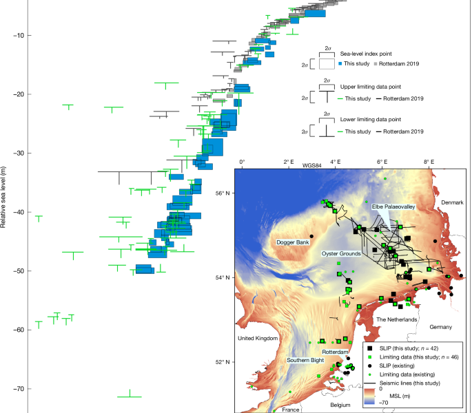
Source: Global sea-level rise in the early Holocene revealed from North Sea peats

Uncertainty in obsrsl between 11 ka and 3 ka: Estimating residual RSL change with EIV-IGP model 37,38

The uncertainty in obsrsl is taken from the HOLSEA database, whereas for average[pEuIS], the standard deviation calculated from the eight GIA models is used as a measure of uncertainty. From the resulting data series (supplementary information49 section 4), we calculated residual RSL and rates of residual RSL change with the EIV-IGP model37,38 (Extended Data Fig. 9), showing 26.3 m (2σ range, 23.8–28.8 m) of residual SLR for the 11–3 ka period (Fig. 4a).

To calculate the contribution of the AIS to GMSL, we used recent ensembles of deglacial simulations that are constrained by geological observations12. We used the ten top scoring simulations highlighted in that paper to calculate the median contribution from the AIS of 7.8 m SLE between 11 ka and 3 ka. The calculation shows 8.1 m SLE for the duration of the entire Holocene. The simulations show that the AIS was smaller than it is now.

There are additional details and references regarding the methods.