Automated segmentation of cortical image using distributed watershed clustering algorithm based on a convolutional network and tissue map
The image segment is described in the ref. 62. Remaining misalignments were detected by cross-correlating patches of image in the same location between two sections after transforming into the frequency domain and applying a high-pass filter. Combining with the tissue map previously computed, a ‘segmentation output mask’ was generated that sets the output of later processing steps to zero in locations with poor alignment. Using previously described methods68, a convolutional network was trained to estimate intervoxel affinities that represent the potential for neuronal boundaries between adjacent image voxels. A network was trained to classify the image into five categories: nucleus, dendrite, glia, and blood vessel. It is recommended that you follow the methods described in ref. 69, both networks were applied to the entire dataset at 8 × 8 × 40 nm3 in overlapping chunks to produce a consistent prediction of the affinity and neurite classification maps, and the segmentation output mask was applied to predictions. The affinity map was processed with a distributed watershed and clustering algorithm to produce an oversegmented image, where the watershed domains are agglomerated using single-linkage clustering with size thresholds70,71. The final segmentation was created by using a distributed mean affinity clustering scheme.
For every proofread cell in the cortical column (described above), we compared the cellular volume of the initial reconstruction from the automated segmentation to the cleaned and completed reconstruction. To measure the precision connectivity for each cell, we noted the number of synapses that got removed with proofreading, the number of synapses that were added, and the number of synapses that were maintained with each cell before and after proofreading.
Using these boundaries and nucleus centroids5, all cells were identified inside the columnar volume. The classification of cells was assigned on the basis of a brief manual examination and later checked by the newer versions of the classification described here. To facilitate concurrent analysis and proofreading, all false merges that connected any column neurons to other cells (as defined by detected nuclei) were split.
We began by looking at all the branch points for false axons. We then performed extension of axonal tips until either their biological completion or data ambiguities, particularly emphasizing all thick branches or tips that were well-suited to project to new laminar regions. For axons with many thousands of synaptic outputs, we followed many but not all tips to completion once primary branches were cleaned and established. Most tips were extended to the point of completion or ambiguity for smaller neurons. The amount of time it takes for axons to be written was different by cell type but also by axon thickness that resulted in higher quality autosegmentations. Typically, inhibitory axon cleaning and extension took 3–10 h per neuron.
Basket cells are cells that make 20% of theirsynaptic inputs onto the soma or dendrites of cells. Neurogliaform cells were recognized by having a low density of output synapses, and boutons that often had synaptic vesicles but no postsynaptic structures. The cells were labelled by having 2 or 3 dendrites, and mostly making s— with other people’s cells. The Martinotti/non-Martinotti subclass label has been given to cells that are capable of targeting the peripheral dendrites of excitatory neurons without having hallmark features of neurogliaform cells.
Dendritic extents and neural network targeting of cells measured in the MICrONS dataset, with applications to Chandelier cells and axo-Xonal neurons
The training set was augmented with manually labeled errors from the whole dataset because of the high levels of editing in the column.
To estimate the likelihood of truncation, we measured the distribution of dendritic extents from the proofread column cells. For each cell, we measured the radial distance of each input synapse from the cell’s soma. The 97th percentile of the distribution was defined when calculating the distance from the soma of every input synapse for each cell. If the median value was less than 250 m we could use it as a threshold for truncation, but if it was more than that we would need to guarantee truncation for any cell. For the rest of the cells in the dataset, we measured the distance of the soma from the volume borders in x and z. The overlap in these distributions relates to the probability of truncation, leading to our conclusion that roughly one-third of the cells have some degree of dendritic truncation.
A neural network was trained to predict if a voxel participated in a nucleus. Following the methods described in ref. This map was created on the entire dataset at a maximum of 64 64 x 40 nm3.
To measure the predicted cell densities per subclass across the MICrONS dataset, we divided the dataset into 50-µm2 bins in the x–z plane. For each bin, we calculated the number of cells in each subclass and scaled that value to the number per square millimetre to facilitate direct comparisons to reported densities in the literature.
To quantify whether a cell preferentially targeted 5P-NP neurons, we measured the fraction of total output that targeted different predicted subclasses. There is a rare preferences for cells that output more than 30% of their synapses onto 5P-NP cells. A two-tailed Fisher exact test was carried out to test significance between the random cell population and the nearest neighbours.
Chandelier cells have unique axo-Xonal synapses that are found on the AIS of pyramidal cells. As there were no chandelier cells within the densely reconstructed column, we sought to test whether the perisomatic feature space would facilitate an enriched dataset-wide search for these cells. After selecting the 20 nearest neighbours by distance from the chandelier cell we used a KDTrees search of the perisomatic feature space to find the best ones. Random cells from the predicted inhibitory neurons were selected. For each of these 40 cells, we proofread the reconstructions to ensure that there were no extraneous neurites attached, and extended the axon until there were at least 100 output synapses. On average, each of the 20 nearest neighbours had 590 output synapses attached and the random cells had 809 synapses attached.
The hierarchical model was defined as the sequential combination of the best-performing classifiers at each level. The performance of different feature sets is shown in the table. The performance of the hierarchy model was measured with a test set that was used to inspect 100 examples of each of the subclasses as well as errors. The test set of 1,700 cells was created by this. The results of cross-validation and test performance are reported. All scores reported are based on the sample rate for each class in the column.
The model type for each of the following classifiers was chosen based on a randomized grid search for the following models: support vectors machine with a linear kernel, support machines with a radial basis function and nearest neighbours. The top-performing model was chosen based on the training parameters for each type. Individual models were further optimized using a measure for recall and precision, called the F1 score. Training and test examples were held to the same standards.
Given a cell for which all PSSs have been extracted within a 60 µm radius from the nucleus centre, the objective was to build a descriptor that encapsulates the various properties of the PSS. In particular, we aim to capture two of these properties: the type of shape of the PSS and the distance of the PSS from the soma. We needed a representation for each cell based on the number ofapses and their shapes. To capture shape information, a dictionary of all shape types was built using a dictionary dataset from 236,000 PSSs from a variety of neurons24. The shapes were normalized to make way for the autoencoder 60,61, which learned a representation of size 1,024. The high-dimensional latent space spanning all of these shapes is a continuous space (Extended Data Fig. 3), which was used to generate a bag of words model30 for the shapes. To ensure that we were sampling the entire embedding space, we carried out k-means clustering with k = 30 to estimate cluster centres. We manually reordered the bin centres for visualization purposes from shapes representing small spines, to those representing longer spines, to dendritic shafts of different shapes, and finally somatic compartments. The top row of the right panel of Fig. 4d shows the shape in the dictionary that is closest to each of these cluster centres. For distance from the soma, we split the 60 µm radius around the nucleus centre into four 15-µm radial bins (Fig. 4c,d). The PSSs were binned based on their shape and distance. We started by getting PSSs from within 120 m. The additional radial bins did not increase our differentiability and so we reduced the radius to 60 m. The other features were added to the Z-scored histogram and then added to the UMAP embedded in the other features.
The mesh around the 3,500- nanometer region was obtained through the sphinx region. The smaller cutouts resulted in some confusion in the identification of the main shaft and caused some errors in the skeletonization. The skeletons were more stable and as expected, at 3,500nanometers. The mesh was then divided by using the CGAL surface segments method which splits the regions on the basis of thickness. The PSS region was identified by using a local skeleton calculated from the synep region mesh, not the whole-cell mesh. This allowed us to adapt this method for cells in the dataset without the need for proofreading.
For 2D UMAP embeddings and training of the classifiers, it was important to place all features in approximately similar scales. For this reason, we independently z-scored each feature across all cells and used that as the input for classifier training as well as the UMAP embeddings in Figs. 3–6.
Visualization of MET-types across the whole-brain taxonomy using Kruskal-Wallis and Conover post hoc tests
Comparisons across several MET-types were performed using non-parametric Kruskal–Wallis tests followed by Conover post hoc tests with Bonferroni corrections for pairwise comparisons. If Kruskal–Wallis P values 0.05 and post hoc tests for pairwise comparisons are P 0.05, the values are indicated on plots. Errors reported are s.e.m. unless otherwise indicated. Comparisons of the fraction of cell types targeted by a MET-type (from 0 to 300 µm) (Fig. 3a) were performed using a non-parametric Kolmogorov–Smirnov test with P values adjusted by a false discovery rate (Benjamini–Hochberg) correction. The boxplot whiskers indicate the maximum/minimum range of data, with n being 173 inhibitory neuron from the EM dataset and n being 16 extended MCs. The cells are measured several times.
We compared the differentially expressed genes with the main transcriptomic types using the scrattch.hicat. Sst Cbln4 and MET-4: Sst Calb2 Necab. Sst Calb2 Pdlim5; Sst Chrna2 Ptdg4 is MET6. Sst Myh8 and Sst Myh8 Etv To identify the pairswise differentially expressed genes, they looked for genes with at least a twofold change in expression and an adjusted P value of less than 0.02. The top five upregulated and downregulated genes for each pairwise comparison were selected for visualization (ranked by adjusted P value). The average expression of these genes and the fraction of cells with non-zero expression was calculated and presented as a dot plot for the three Sst MET-types. Only genes expressed in at least 50% of cells in at least one MET-type were selected for visualization.
Proportions of MET-types were estimated from a recently published MERFISH dataset67. Cell counts were calculated for each Sst t-type in VISp in the MERFISH dataset. We identified correspondences between t-types across several taxonomies as the cells were mapped to a whole-brain taxonomy67. In order to identify the Tasic et al.6 t-types that have the highest number of shared cells, we first needed to find the original taxonomy of Tasic et al.6. The whole-brain Taxonomy and the CTX/ HPF had their correspondences taken directly from ref. 66. We assigned Tasic et al.6 t-types to the MET-types to which the largest number of cells belonged16, except for the t-type Sst Calb2 Pdlim5, for which corresponding cells were assigned to either Sst MET-3 (if located in L4 or above) or Sst MET-4 (if located in L2/3). The cells from the Sst MET-1 subclass were not analysed here. A small number of cells were contained in the original study16 but no clear t-type correspondences were found.
Using automatically detected synapses, annotators visualized all output synapses on a given presynaptic cell in Neuroglancer. Regions lacking synapses were manually inspected in the EM imagery. If myelination was seen, an annotator marked the start and end point of each myelinated segment in Neuroglancer to generate a line. The number of these annotations was summed to determine the number of myelinated segments per cell. The length of each annotation was summed to determine the distance of myelinated axon per cell.
For 500 iterations, a random subsample (95%) of the Patch-seq data was selected with probabilities according to MET-type class size (a Patch-seq cell from a well-represented MET-type was more likely to be omitted). MET-types with 5 or fewer specimen were exempt from subsampling. In each iteration, a new RFC with the aforementioned parameters was fitted with sub-sampled Patch-seq data and MET labels were predicted for EM cells. The final MET assignment was given as the most frequently predicted MET label for each cell (Extended Data Table 1). We used these predicted MET-type labels to group cells for subsequent analysis.
The mean and s.d. of the Patch-seq data were used to calculate the z scores.
A reliability metric was quantified as the fraction of iterations each sample was predicted as its final MET assignment out of all predictions (for example, a cell was predicted into this MET-type 80% of the time). To find the right threshold, we looked at reliability scores in the data. We applied random subsampling iterations in a leave-one-out manner to the Patch-seq data. We set one sample aside and use the rest for training. In each iteration, the training data are sub-sampled randomly as described above and used to fit a new RFC. The label of the single left-out patch-seq sample is predicted by the analysis of the classifier. After this process was done 500 times each cell had a predicted reliability metric and label. We plotted a cumulative histogram of the correctly and wrongly predicted labels. We found that a reliability score of more than 0.54 is the most inclusive value at which Patch-seq samples are more frequently predicted correctly than incorrectly (Extended Data Fig. 2b).
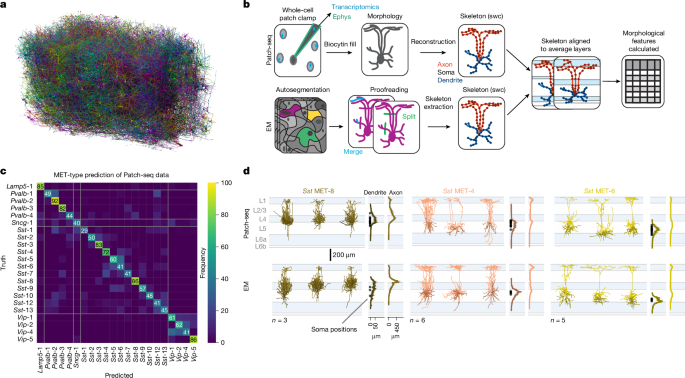
The performance of the support vector machine and logistic regression model was assessed for predicting MET-type labels for Patch-seq cells using the features of inhibitory cell types from a previously published Patch-seq dataset. The method we used to assess classification accuracy is a fivefold cross-validation approach. The data were split randomly into five partitions while maintaining the distribution of MET-type labels in each partition. The method iteratively rotates which partition is held back from training and used to check the model. MET-types with fewer than five morphological reconstructions (Lamp5 MET-2, Pvalb MET-5, Sncg MET-2, Sncg MET-3, Sst MET-11 and Vip MET-3) were omitted. The maximum depth of ten, balanced class weights, minimum of ten samples per split and at least five samples per leaf match the results of a support vector machine model. Fivefold stratified cross-validation with shuffling was repeated 20 times and achieved a mean accuracy of 58.9 ± 4.1% (s.e.m.), far exceeding the expected chance accuracy for 22 categories (4.5%). Classifier accuracy was determined by how frequently the model correctly predicted the MET-type label of held out data (not used in training the model) (Fig. 1c and Extended Data Fig. 5a). We calculated an overall F1 score of 0.58, based on averaging F1 scores for each MET-type, based on classifying that type versus any other type. The cumulative confusion matrix for hold-out validation data was recorded. 1c.
Each mesh underwent skeletonization to create a list of branch and end points. Each branch point was inspected manually. True branch points were left alone and false branch points (often due to overlapping processes from distinct cells) were split using Neuroglancer tools. Each end point was inspected manually. True endpoints were left alone and false endpoints (premature end of a process) were extended by an expert annotator, who would follow the process along the EM imagery to a natural ending (bouton, tapered end) or until the process could no longer be extended reliably (for example, edge of block). The number of reconstructions of the cells used in the study is 173.
We restricted the number of synaptic outputs on the axon of the inhibitory neuron as we did not find any correctly categorized synaptic outputs on the arbour. One cell with fewer than 30 synaptic outputs was omitted because of insufficient size. All interneurons’ synaptic outputs were kept out of the column unless otherwise specified. The target skeleton, dalen, and M-type of the target neuron were also tagged with the outputs on the basis of the definitions above.
The number of multisynaptic connection connections that were within 15 m of each other as well as the target were measured. The results of our evaluation suggest that intersynapse distances of 5 to 100 m have the same results.
Using these six features, we trained a linear discriminant classifier on cells with manual annotations and applied it to all inhibitory cells. Differences from manual annotations were treated not as inaccurate classifications but rather as a different view of the data.
Tortuosity and k-means clustering in excitatory M-types from a connectomic census of mouse visual cortex
There is a path that goes from branch tips to soma per cell. Tortuosity is measured as the ratio of path length to the Euclidean distance from tip to soma centroid.
There is a median linear density. This was calculated by taking the net path length from layer 1 to white matter, and dividing it by 50 to calculate the median. A linear density was found by dividing synapse count by path length per bin, and the median was found across all bins with non-zero path length.
The features were computed after a rotation of 5 degrees to flatten the pial surface and translations to set it at 0 on the y axis. It was not made clear that features on the basis of apical classification were not specifically used to avoid ambiguities.
To find out the significance of each feature for each M-type, we trained a random forest classifier and used scikit-learn78. SMOTE resampling was used to get more datapoints from the smaller class. We used the Mean Decrease in Impurity metric to determine how often a feature was used.
We used the number of synapses across all excitatory M-types to get the number of interneurons for the clustering. The synaptic output budget was normalized to create aVector for each neuron with elements ranging from zero to one. The number of times two cells were put in a single k-means cluster was used to divide the normalized synaptic output budgets. A final value of 18 was found by clustering with complete linkage and using a silhouette score and a Davies-Bouldin score, as well as scanning outputs from two to 25 clusters.
Source: Inhibitory specificity from a connectomic census of mouse visual cortex
Synaptic cleft detection and assignment using an autoTEM dataset with shuffled selectivity index of Layer 6 pyramidal cells to M-type
On the basis of compartment, we can see a very similar selectivity index to that shown on M-type cards. In that case, the shuffled distribution preserves observed depth and M-type output distributions but not compartments.
For synapse detection and assignment, a convolutional network was trained to predict whether a given voxel participated in a synaptic cleft. Inference on the entire dataset was processed using the methods described in ref. 69 using 8 × 8 × 40 nm3 images. These synaptic cleft predictions were segmented using connected components, and components smaller than 40 voxels were removed. A separate network was trained to perform synaptic partner assignment by predicting the voxels of the synaptic partners given the synaptic cleft as an attentional signal72. This assignment network was used to identify clefts, and the coordinates of both the presynaptic and postsynaptic partner predictions were Logied along with each cleft prediction.
The curvature is not aligned to a sectioning plane or associated with shearing or other distortion in the imagery, making it unlikely to be a result of the alignment process.
It is unlikely that the blood vessels have a large, correlated distortion in deep layers. Moreover, it is unclear why such stress would affect only layer 5b and below.
Similar curvature has been observed in other large EM datasets from visual cortex (data not shown) and light level morphological reconstructions, particularly among layer 6 pyramidal cells.
The volume assembly line up is described in detail. Briefly, the images that the autoTEMs pick up are first corrected for distortion effects by using a set of 10 10 highly overlap images. Overlapping image pairs are identified in each section, as well as point correspondences and features that have been created using the scale-invariant feature transform. The sum of squared distances between the point correspondences of these tile images is normalized with the help of the maximization of the montage transformation parameters. A downsampled version of these stitched sections is produced for estimating a per-section transformation that roughly aligns these sections in three dimensions. The rough aligned volume is rendered to disk for further fine alignment. There is a software tool that can be used to Stitch and Align the dataset. To fine align the volume, we needed to make the image processing pipeline robust to image and sample artefacts. Cracks larger than 30 um (in 34 sections) were corrected by manually defining transforms. The smaller and more numerous cracks and folds in the dataset were automatically identified using convolutional networks trained on manually labelled samples using 64 × 64 × 40 nm3 resolution images. The same was done to identify voxels containing tissue. An approach based on a convolutional network was used to estimate the displacements between two images. The final displacement field was created for each image by combining the estimated displacement fields from the adjoining sections. First, alignment was refined by using 64 64 40 nm3 images. The composite image of the partial sections was created using the tissue mask previously computed.
The study used a fleet of transmission electron microscopes that had been converted to continuous automated operation. It was built on a standard JEOL 1200EXII 120 kV transmission electron microscope that had been modified with customized hardware and software, including an extended column and a custom electron-sensitive scintillator. A low-distortion lens was used to grab the frames from a single large-format camera that averaged 100 ms per frame. The autoTEM had a sample stage that offered high-fidelity montaging of large tissue sections, and a system that locates each section using index barcodes. During the procedure, the reel-to-reel GridStage moved the tape and discovered the targeting area through its barcode. Quality controls were performed on the re image sections that failed the screening.
Candidate mice were shipped via overnight air freight to the Allen Institute after they were read at the College of Medicine. 2.5% paraformaldehyde, 1%glutaraldehyde, and 2 mM calcium chloride were used to percise the mice in an 0.08 M sodium cacodylate buffer. A thick (1,200 µm) slice was cut with a vibratome and post-fixed in perfusate solution for 12–48 h. Reduction of osmium treatment is based on the protocol of ref. 64. All steps were done at room temperature. The first osmication step involved 2% osmium tetroxide (78 mM) with 8% v/v formamide (1.77 M) in 0.1 M sodium cacodylate buffer, pH 7.4, for 180 min. Potassium ferricyanide 2.5% (76 mM) in 0.1 M sodium cacodylate, 90 min, was then used to reduce the osmium. The second osmium step was at a concentration of 2% in 0.1 M sodium cacodylate for 150 min. Samples were washed with water and then immersed in thiocarbohydrazide for further intensification of the staining (1% thiocarbohydrazide (94 mM) in water, 40 °C, for 50 min). Samples were immersed in 2% water for 90 minutes after washing with water. After washing in the water, a buffer of lead nitrate and aspartate was used to enhance the contrast. The samples proceeded through a graded dehydration series of 50%, 70%, 90% w/v in water, 30 min each at 4 C, then 3 100%, 30 min each at room temperature. Two rounds of 100% acetonitrile (30 min each) served as a transitional solvent step before proceeding to epoxy resin (EMS Hard Plus). A progressive resin infiltration series (1:2 resin:acetonitrile (for eample, 33% v/v), 1:1 resin:acetonitrile (50% v/v), 2:1 resin acetonitrile (66% v/v) and then 2 × 100% resin, each step for 24 h or more, on a gyrotary shaker), was done before final embedding in 100% resin in small coffin moulds. Epoxy was cured at 60 °C for 96 h before unmoulding and mounting on microtome sample stubs. The sections were then collected at a nominal thickness of 40 nm using a modified ATUMtome (RMC/Boeckeler61) onto six reels of grid tape61,65.
The animal procedures were approved by the Institutional Animal Care and Use Committee at the Allen Institute for Brain Science. Data acquisition was done at the College of Medicine. Afterwards the mice were transferred to the Allen Institute in Seattle and kept in a quarantine facility for 1–3 days, after which they were euthanized and perfused. All results described here are from a single male mouse, age 64 days at onset of experiments, expressing GCaMP6s in excitatory neurons via SLC17a7-Cre and Ai162 heterozygous transgenic lines (recommended and generously shared by Hongkui Zeng at the Allen Institute for Brain Science; JAX stock 023527 and 031562, respectively). Between P80 and P75 two-photon functional and structural images were taken of the cell bodies and blood vessels. The mouse was perfused with blood.
Source: Inhibitory specificity from a connectomic census of mouse visual cortex
The MICrONS dataset: Accurate alignment, segmentation and data flow. I. Data analysis methodology and the primary resource for the dataset
This dataset was acquired, aligned and segmented as part of the larger MICrONS project. Methods underlying dataset acquisition are described in full detail elsewhere2,61,62,63, and the primary data resource is described in a separate publication2. We repeat some methodological details here for convenience.