Mapping the ULE Database for Extreme Weather Events with Pre-Industrial Lifetime Exposures based on ISIMIP2b Simulations
The past decade has been identified as being among the ten hottest years recorded in two centuries of observations. This anthropogenic climate change is driving not only an increase in the intensity and frequency of extreme weather events, but also changes in the spatial and temporal distribution of such events. For instance, wildfires in Siberia2 and severe floods in Libya have both occurred in the past few years but were historically rare or absent. Extreme weather events are taking place earlier, later or more frequently in the year, their duration is increasing, and historical seasonal patterns are being disrupted, due to storms hitting outside their usual seasons. Previously unprecedented events have become part of present-day reality.
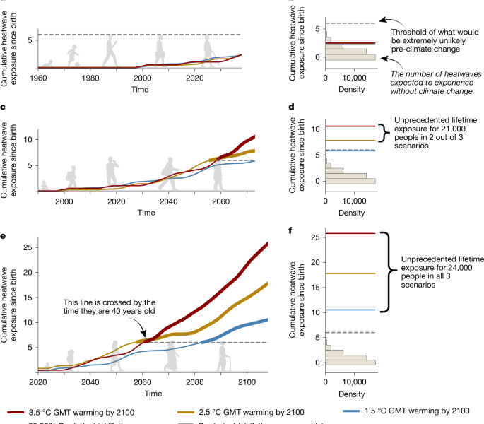
To generate a baseline distribution of lifetime exposure in a world without climate change, large samples of pre-industrial lifetime exposures are bootstrapped assuming 1960 life expectancy in each country. Here, for each exposure projection originating from a simulation under a pre-industrial climate, 10,000 lifetime exposures are estimated by resampling exposure years with replacement. Depending on ISIMIP2b data availability, pre-industrial exposure projections have a length of 239–639 years per simulation from which to resample from11. This process generates 40,000–310,000 country-wide maps of lifetime exposure, depending on the extreme event considered and its underlying data availability, enabling exposure projections in a pre-industrial climate. Using the pre-industrial period as a baseline enables (1) our GMT mapping procedure; (2) bootstrapping a stationary time series to achieve a large reference dataset; and (3) the production of a reference dataset with information that is independent of the projections forming our ULE estimates.
Every year, all demographic datasets are changed to represent lifetimes. When calculating life expectancies, the first step is to assume that the values of the original 5 year groups are representative of the middle group. The life expectancies are added to capture the life expectancy of the cohort since birth when the data begin at age 5. The maximum life expectancy for people who were born in 2020 must be assumed to be 2113, which is the final year of the analysis. For population totals, we take each year beyond 2100 as the mean of the preceding 10 years of the dataset, such that population numbers for 2101 are the mean of 2091–2100. To maintain the original population sizes, we interpolate annual cohort sizes and age groups from the original five-year age groups and divide age totals by 5. This provides the absolute numbers of 0- to 100-year-olds for each year across 1960–2113.
Impact model comparison between urban areas and grid-scale datasets using an ISIMIP2b model of climate change based on bias-adjusted global climate models
The Inter-Sectoral Impact Model Intercomparison Project (ISIMIP) provides a simulation protocol for projecting the impacts of climate change across sectors such as biomes, agriculture, lakes, water, fisheries, marine ecosystems and permafrost (www.isimip.org). In ISIMIP2b, impact models representing these sectors are run using atmospheric boundary conditions from a consistent set of bias-adjusted global climate models (GCMs) from phase 5 of the Coupled Model Intercomparison Project (CMIP5) that were selected based on their availability of daily data and ability to represent a range of climate sensitivities17; the Geophysical Fluid Dynamics Laboratory Earth System Model (GFDL-ESM2M; ref. 30), the earth system configuration of the Hadley Centre Global Environmental Model (HadGEM2-ES; ref. 31), the general circulation model from the Institut Pierre-Simon Laplace Coupled Model (IPSL-CM5A-LR; ref. 32) and the Model for Interdisciplinary Research on Climate (MIROC5; ref. 33). Impact simulations are run for pre-industrial control (286 ppm CO2; 1666–2099), historical (1861–2005) and future (2006–2099) periods. Future simulations are based on Representative Concentration Pathways (RCPs) 2.6, 6.0 and 8.5 of GCM input datasets. Estimations of global exposure to each extreme event category are based on impact simulations and GCM input data. For the full details of these computations, we refer to ref. 12, but we summarize extreme event definitions below.
We use grid-scale indicators of vulnerability to compare with estimates of ULE. The first is an ISIMIP2b GDP input dataset using concatenated historical and SSP2 time series covering 1860–2099 annually17. This dataset was disaggregated from the country to grid level using spatial and socioeconomic interactions among cities, land cover and road network information and SSP-prescribed estimates of rural and urban expansion46. The Global Gridded Relative Deprivation Indexv.1 is a tool to find out the relative deprivation levels between the poor and the rich. This deprivation score uses six input components. The child dependency ratio is the ratio of the population of children and the working-age population. This can indicate vulnerability, for which high ratios indicate a dependency of supposed consumers and non-producers on the working-age (producing) population47. Second, infant mortality rates (IMR), taken as the deaths in children younger than 1 year of age per 1,000 live births annually, are a signal of population health and form a long-term Sustainable Development Goal of the United Nations48. Third, the Subnational Human Development Index (SHDI), an assessment of human well-being across education, health and standard of living, originates from the Human Development Index, the latter of which is considered one of the most popular indices to assess country-level well-being. The HDI is improved in terms of spatial scale and in representation of 161 countries across all world regions. High deprivation is caused by the low values in the ratio of built up to non built up area. The mean and slope of nighttime light intensity are used to indicate deprivation in areas of low nighttime light intensity by the fifth and sixth components. There are components that range from 30 to 1 km in resolution and can be combined into a 0 to 100 range to represent low to high deprivation. For the final aggregation, the IMR and SHDI components are given half the weight of the rest of the inputs, given their coarser resolution. Generations face deprivation and vulnerability to climate extremes through the multiple dimensions of the GRDI. Our approach to vulnerability does not account for real or potential adaptation to climate change, but it gives relevant information on the current adaptation potential of local populations.