Ref. 19F14C and DIC and CO2 from England, Scotland, and Peru, taken from the PKU_AMS facility in 2017 and 2018

To understand the relationship between F14C and DIC and CO2 emissions, we took 15 measured F14C data and combined them into a table. These paired samples cover 11 distinct sites and a river pH range of 4.2–7.7, indicative of the range of pH found in natural waters. Six of these observations come from ref. 19 which was taken from two headwater streams in England and Scotland. In addition, there are also measurements obtained from the headwater streams of the north of Scotland and the Flow Country. Another unpublished paired measurement was obtained from Peru, from the Manu River. Sample 14C collection and processing for the new Scotland and Peru measurements were the same as for the London, Taiwan and Cambodia samples outlined above.

Samples collected in 2017 and 2018 were processed and analysed at the Peking University AMS facility (PKU_AMS) in Beijing, China, following ref. 59. Water samples were acidified and heated to 75 C for 2 hours to convert DIC to CO2. The CO2 was then purified cryogenically on a vacuum line and graphitized using zinc reduction. The samples were analysed in Miami, Florida, USA. Samples were acidified using phosphoric acid and stripped from the water by bubbling pure N2 or Ar gas through the sample. The resulting CO2 was collected cryogenically and graphitized using hydrogen reduction of the CO2 sample over a cobalt catalyst. In both the PKU and Beta labs, reference standards, internal QA samples and backgrounds were processed alongside the samples.

Owing to inconsistencies in how catchment characteristics were reported in the literature from which we assembled the radiocarbon measurements (if they were reported at all), we used a global database of hydrological-environmental characteristics (HydroATLAS56) to extract key catchment information for each sampling location in a consistent manner (for example, catchment size, lithology, biome).

Tropical broadleaf and conifer forests, which included HydroATLAS biomes ‘1. Tropical & Subtropical Moist Broadleaf Forests’, ‘2. Tropical & Subtropical Dry Broadleaf Forests’ and ‘3. Tropical & Subtropical Coniferous Forests’.

A new age and uncertainty 61 for the atmospheric F14C-CO2 sample collected more than four times in the year of sample collection and removed from the database

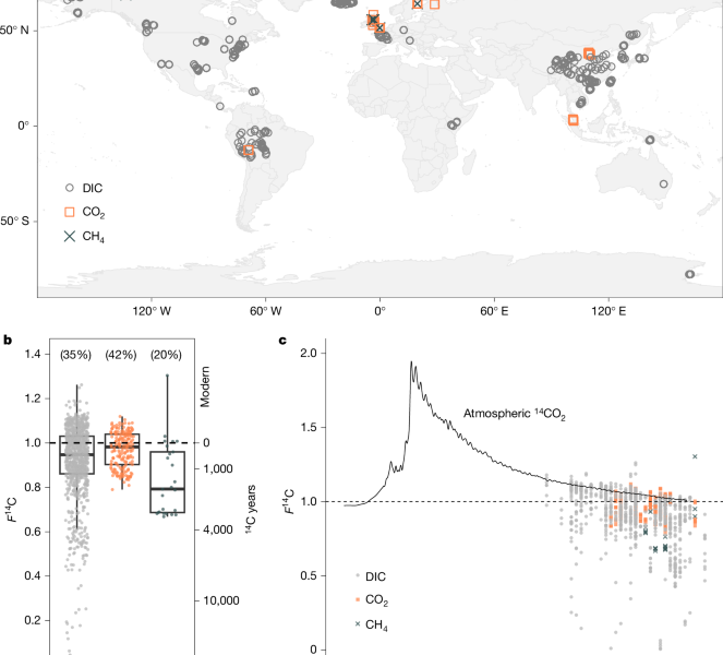
We normalized the values in the database for each measurement into the F14C-CO2 level in the atmosphere in the year of sample collection.

Some locations in a database were visited more than once. This is also because of the combination of experimental approaches such as repeat sampling and exploration of temporal variations. When a sample location was repeat sampled more than four times in a calendar year (that is, more than 0.5% of all observations), we took the average of the F14C observations at that location for that year and recalculated a new radiocarbon age and uncertainty61. This removal left a total of 1,020 observations.

Source: Old carbon routed from land to the atmosphere by global river systems

DIC Samples from Taiwanese Rivers and the Mekong River in Cambodia deposited into a 1-L Foil Bag

River water DIC samples from Taiwanese rivers and the Mekong River in Cambodia were collected using the methods outlined in refs. It was 18,58. In Taiwanese rivers, 1-l sampling bottles were submerged into the middle of the channel using a weighted Teflon sampler. On the river, near-surface samples were collected with a Niskin-type sampler. The river water was then fed through the polyethersulfone filters into preweighed 1-L foil bags, with care to avoid atmospheric air mixing. The foil bag was filled with around 200–500 liters of river water and gently squeezed before closing to ensure that no air was trapped. During fieldwork, the filled bag was reweighed and stored at 4 C before it was shipped to the UK where the sample was frozen within a week.

Sedimentary, which included the HydroATLAS classes ‘1. Unconsolidated Sediments (SU)’, ‘3. There are Siliciclastic Sedimentary Rocks. Mixed Sedimentary Rocks (SM)’ and ‘6. Carbonate Sedimentary Rocks (SC)’.

One data point returned ‘No Data (ND)’ from the HydroATLAS lithology classes and was excluded from the lithology analysis. Data from Antarctica were also excluded from the analysis owing to a lack of lithology data (returning ‘Ice and Glaciers (IG)’ from the HydroATLAS lithology classes).

Source: Old carbon routed from land to the atmosphere by global river systems

Random Forest Modelling of HydroATLAS-F14Catm Data: Statistical Analysis of the Relationship between River Carbon Emissions and Input Variables

Statistical analyses were carried out in R version 4.1.1 (ref. 63). We used nonparametric Kruskal–Wallis tests with the kruskal.test function in R, supplemented by post hoc analyses consisting of Conover–Iman tests using the conover.test function and unpaired two-sample Wilcoxon tests using the wilcox.test function. The lm function is used for linear regression analyses. The details of where each analysis is applied are provided in the Figures in the main text, Extended Data and Supplementary Information.

We explored the possible reasons for the age of river carbon emissions using a random forest model. Random forests are a machine learning model that integrate numerous regression trees to make predictions. It has been found that this approach has been successful in unraveling the interplay among variables in environmental studies due to its ability to capture relationships and mitigate the risk of data overfitting. In this study, we use random forest models to investigate the relationships between key catchment characteristics extracted from HydroATLAS and F14Catm values in the database. We wanted to identify which variables had the best control on river carbon emissions.

To avoid the results being influenced by correlated input variables, we removed variables that correlated significantly with other potential input variables based on Spearman correlation greater than 0.6. The remaining variables are shown in Supplementary Table 5 and includes the year of sample collection (‘year’).

We split the model runs by catchment size (Extended Data Figs. 3 and 4) using whole catchment characteristics for rivers with catchments greater than 10 km2 and reach characteristics for rivers with catchments ≤10 km2. Owing to limits on the number of data points, we only applied the model to DIC data, in which observations were n > 100 when separated by size.

Source: Old carbon routed from land to the atmosphere by global river systems

Global analysis of F14Catm based on partial dependence analysis of random forest models and estimates of carbonate and rock organic carbon weathering sources

We looked at the association between predictor variables and F14Catm using partial dependence plots. The plots show the change in F14Catm with a given input variable changes but all other variables are unchanging. We performed the partial dependence analysis ten times (mirroring the ten iterations of random forest models from using tenfold cross-validation) and plotted the mean values from these ten runs, with the variability across the runs indicated by the shaded area (Extended Data Figs. 3 and 4).

In a perfect world it would be possible to account for the input of DIC and CO2 from each Watershed in the database. To do this, we need dissolved cation data, as well as anion data and the weathering acids and contributions of carbonate and rock organic matter. Unfortunately, most of the studies reporting river DIC and CO2 F14C measurements do not report dissolved ion data, or if they do, do not report the necessary range of cation and anion measurements to complete a weathering-source inversion. As such, we take a global view using our mean F14C DIC values and assess the petrogenic inputs using global estimates of carbonate and rock organic carbon weathering rates.

$${\rm{Total\; river\; DIC\; flux}}\times {F}^{14}{{\rm{C}}}{{\rm{river}}}=({\rm{lateral\; DIC\; export\; to\; ocean}}+{{\rm{vertical\; CO}}}{2}\,{\rm{emissions\; flux}})\times (a\times {F}^{14}{{\rm{C}}}{{\rm{decadal}}}+b\times {F}^{14}{{\rm{C}}}{{\rm{millennial}}}+c\times {F}^{14}{{\rm{C}}}_{{\rm{petro}}})$$

$$\begin{array}{l}{F}^{14}{{\rm{C}}}{{\rm{river}}}\,\times \,2.5={F}^{14}{{\rm{C}}}{{\rm{decadal}}+{\rm{millennial}}}\,\times \,(2.28\,{\rm{to}}\,2.35)\ \,\,\,\,\,\,\,+\,{F}^{14}{{\rm{C}}}_{{\rm{petro}}}\times (0.15\,{\rm{to}}\,0.218)\end{array}$$

We can then calculate the non-petrogenic F14C value (F14Cdecadal+millennial), because the petrogenic source is assumed to contain no radiocarbon (that is, F14C = 0.0). The F14CDecadal +millennial was given an estimate of 1.078 to 1.007.

We were not able to collect site specific concentration and emission flux data from the literature. This means that we were not able to scale the F14C values in the database with local and regional emission fluxes (Supplementary Information section 4).