Studying the relationship between a paper’s pivot size and impact using binned scatterplots and student’s t-tests

The researchers found that, the larger the pivot size, the less likely a paper is to rank among the top-5% most-cited papers published in its field that year. They also determined that it was more difficult for scientists to get their papers published after a pivot (see ‘When risks don’t pay off’).

When I am giving a researcher, p and t are used to indicate a paper or patent and time is used to indicate a patent application. Observations are at the paper-by-researcher level. We took a non-parametric approach after allowing for potentially Nonlinear relationships between pivot size and impact. Specifically for Extended Data Fig. 1, we generated bins of pivot size and included indicator dummies for a work appearing in the relevant bin. Stata has a large number of individual fixed effects and we ran them in the commands of the reghdfe. There are standard errors that are clustered. The statistical significance of different pivot-size bin coefficients was calculated using t-tests. For simplicity, we report P < 0.001, but note that with observation counts in the millions, these tests present extremely high t-statistics and extremely low P values.

Dashun Wang, a computational social scientist and co-author of the study, said that it showed the scientific fields that a researcher typically draws from. “If I suddenly cite journals that I haven’t cited before, it’s a sign that I’m doing something different,” Wang says.

When you leave a trusted area, you lose your recognition, according to a science-policy specialist at the University of Manchester. He says that the team evaluated a lot of data.

To reveal potentially nonlinear relationships between pivot size and outcome variables, we use binned scatterplots82. The picture is in fig. 2a, papers are ordered by average pivot size along the x axis and binned into 20 evenly sized groups. Each marker is placed at the mean (x,y) value within each group. Binned scatterplots of raw data are further presented in Figs. 2c,e,f and 4e,g–j, and Extended Data Figs. 2, 3, 5–8 and 10b. Student’s t-tests are used to test mean differences from baseline rates (one sample t-tests) or when comparing outcomes between high and low pivot-size vigintiles (two sample t-tests) in raw data. For simplicity, we report P 0.001, but note that the mean tests tend to reject very high t-statistics and very low P values in common means.

A figure shows how a binned-scatterplot approach was used to divide papers in the year 2020. Also, Fig. The 2020 papers should be split according to criteria, including team size, use of new collaborators and funding. In the picture. We account for some controls. The form is considered to be regression of the form.

rm Impact_rmipt.

where Xi is a vector of control variables with associated vector of coefficients Θ; f(Pivot_sizei) allows for a nonlinear relationship between the outcome and pivot size; and εi is the error term. The control variables are fixed effects for average previous impact, author age, team size, number of new collaborators and an indicator variable for funding. We used two regressions to residualize the pivot size and impact, net of the controls. Figure 4k presents the binned scatterplot for the residualized measures.

where Postipt is an indicator for the period after the shock. The indicator for being in the treatment group is absorbed with an individual’s fixed effect and so does not appear separately in the regression. It’s an indicator of being in the treatment group after the shock and it provides the difference-in-differences estimate. The impact of the external event and the reduced form results for impact are shown in fig. 3b,c. The difference-in-differences plots are presented in fig. 3d,e, showing how the treatment effect evolved before and after the retraction date. The Treat_ Postipt variable and the Postipt variable were replaced with a series of relative year indicators.

Alternative citation-based metrics to detect changes in a paper’s focal or journal’s citations, with an application to the pivot penalty in research

$${{\rm{Pivot}}_{\rm{size}}}{{\rm{ipt}}}={\mu }{{\rm{i}}}+{\gamma }{{\rm{t}}}+\beta {{\rm{Treat}}_{\rm{Post}}}{{\rm{ipt}}}+\gamma {{\rm{Post}}}{{\rm{ipt}}}+{\varepsilon }{{\rm{ipt}}}$$

As presented in the Supplementary Information, we considered numerous alternative citation-based measures. These include smoother (non-binary) outcomes, in which a paper’s citation count is normalized by the mean citation counts to articles in the same field and publication year. We further considered the outcome as the percentile rank of the paper’s citations among all articles published in the same field and year. To consider citation counts over other time frames, we added two, five and ten-year windows. We considered alternative indicators to identify a ‘hit’ paper which was in the upper 10, 5, 1, or 0 percent of all publications in a given field. Additional details and associated robustness tests are provided in the supplementary section.

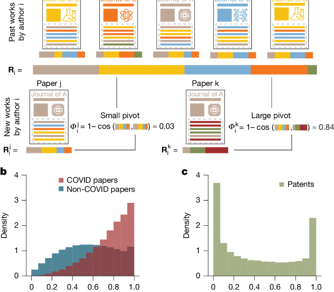
If the focal paper drew entirely on journals from the author’s earlier work, the measure took the value of 0 and the value of 1 if it drew on journals from previous work. The main text has a measure that shows the amount of change in the focal paper compared with the author’s work. We also calculated our measure by using all previous work of a given author, arriving at similar conclusions (Supplementary section 2.2.1 and Extended Data Fig. 10). We looked at the pivot measure based on the fields of the cited references, and found confirmation in our main analyses using it.

Source: The pivot penalty in research

BfR_rmij=1-fracbfPhi4-$p,cdot$(varphi

$${\varPhi }{{\rm{i}}}^{{\rm{j}}}=1-\frac{{{\bf{R}}}{{\rm{i}}}^{{\rm{j}}}\cdot {{\bf{R}}}{{\rm{i}}}}{\parallel {{\bf{R}}}{{\rm{i}}}^{{\rm{j}}}\parallel \parallel {{\bf{R}}}_{{\rm{i}}}\parallel }.$$