Locations of Dm3, TmY and LC15 cells from monosynaptic connectivity maps from Tm1 and Mi1
Locations for Dm3 and TmY cells were computed from maps of monosynaptic connectivity from Tm1. Locations for LC15 and LC10ev cells were computed from their strongest disynaptic pathways, Mi1–T3–LC15 and Tm1–TmY9q–LC10ev. In all cases, the map was convolved with a linear filter that was 1.1 in the central column and 1 in its six neighbouring columns. The maximum of the result was taken as the location of the cell. This centre is often close to the ellipse centre (the centroid of the map), but they are not necessarily the same.
If the origin of the coordinate system is at the B cell, then the normalized number of cells is the average number of synapses received by a B cell from A cells.
We constructed a map of reciprocal connections between neuropils in the form of a triangular matrix with the neuropils as axes. For clarity, here we will refer to a unidirectional connection as an edge. A connection has two opposing edges. Most edges are composed of strontiums in a single neuropil after thresholding. We therefore applied a winner-take-all approach to assigning edges to neuropils. The edge from X to Y is called edge 1 and the edge from Y to X is called edge 2. If the synapses that form edge 1 are in neuropil A, and the synapses that form edge 2 are in neuropil B, then we assign this reciprocal pair to the neuropil A to B square of the matrix. This was done for all reciprocal pairs, with each reciprocal pair is counted as 1 in the matrix. Note that this means that a given neuron can be represented multiple times if it has multiple reciprocal partners.
One Pab is the fraction of inputs to neuron b. Similarly, the matrix PAB is the fraction of input synapses to cell type B that come from cell type A.
Elliptice approximation for receptive fields in lattice-constrained systems: The width of a 1D column
The directions point to next-nearest neighbours which are lattice constant away. The projections grouped hexels with equal q − p, q or p. The resulting coordinate was in units of lattice constant (\times \sqrt{3}/2).
The ellipse approximation is used to estimate the receptive field size. I used a 1D projection onto directions defined on the hexagonal lattice. Each hexel was given coordinates (p, q), with the origin placed at the anchor location used for alignment.
The above has implicitly defined (2\sigma ) as the width of a 1D Gaussian distribution, for which ({\sigma }^{2}) is the variance. It’s the maximum size at a full-width of e 1/2. Alternatively, the width could be estimated by the full-width at half-maximum, (\sigma 2\sqrt{2\mathrm{ln}2}\approx 2.4\sigma ). For either estimate, the width is proportional to (\sigma ). I stick with the simpler estimate (2\sigma ), which can be readily scaled by any multiplicative factor of the reader’s preference.
The first term of the covariance matrix C effectively regards the probability distribution as a weighted combination of Dirac delta functions located at the lattice points. The second term is a correction that arises if each delta function is replaced by a uniform distribution over the corresponding hexagon. This replacement makes biological sense because a column receives visual input from a non-zero solid angle. If there was a single hexel concentrated at a single delta function, the width and length would disappear. With the correction, the length and width of an image with a single non-zero hexel become (s\sqrt{5/3}=a\sqrt{5}/3), in which (a=s\sqrt{3}) is the lattice constant. The correction becomes relatively minor when the length and width of the image are large.
in which I denotes the 2 × 2 identity matrix and s denotes the length of a hexagon side. The length and width of the hexel image are defined as (2{\sigma }{\max }) and (2{\sigma }{\min }), in which ({\sigma }{\max }^{2}) and ({\sigma }{\min }^{2}) are the larger and smaller eigenvalues of the covariance matrix. The approximating ellipse is centred at the image centroid, and oriented along the principal eigenvector of the covariance matrix.
Connectomic properties of the cell types in the central brain of the Fly Fig. v630 snapshot (with an appendix written jointly with Dr. J. B. Sinha)
All analyses presented in this paper were performed on the v630 snapshot of the dataset. The v630 snapshot contains 127,978 neurons and 2,613,129 thresholded connections. The central brain of the fly was thoroughly reviewed, with 80% of it complete. We don’t think the addition of photoreceptors would affect the results of our whole brain network. At the time of publication, the most up-to-date version of the dataset is the v783 snapshot, containing 139,255 neurons, 2,701,601 thresholded connections and completed optic lobes. There are two data snapshots available at Codex.
To look at projections in the 2T-dimensional feature vector is an approach to interpretation. For each cell type, we select a small subset of dimensions that suffice to accurately discriminate that type from other types (Extended Data Fig. 3c. Here we normalize the feature vector so that its elements represent the ‘fraction of input synapses received from type t’ or ‘fraction of output synapses sent to type t’. The total number of input and output synapses is not just the ones with other neurons in the brain.
A companion paper was released with annotations for Dm3, TmY4 and TmY9 cell types, but they were only mentioned in passing. This work is the first to describe the connectomic properties of these cell types.
Line amacrine cells were described in Strausfeld’s Golgi studies of Calliphora and Eristalis1, as well as Musca65. There were also unseen observations of line amacrine cells. Dm3 is a line amacrine cell in a Golgi study.
Light microscopy with multicolour stochastic labelling3 went beyond Golgi studies by splitting Dm3 into two types with dendrite at orthogonal orientations. Dm3p and Dm3q had different transcriptomes when they were younger. (Ref. 18 used the alternative names Dm3a and Dm3b.) Immunostaining showed that Dm3q expresses Bifid, whereas Dm3p does not. Ref. 18 also analysed a reconstruction of seven medulla columns64, with the results showing that Dm3p and Dm3q prefer to synapse onto each other, foreshadowing the present work, and speculatively placed Dm3 cells in the motion pathway.
TmY4 and TmY9 were previously described2. The two TmY9 types can either be distinguished by the directions of the neurites or by their connections. Their stratification profiles are slightly different (Fig. 1a). TmY9q⟂ stratifies in layers 1 and 2 of the lobula plate, whereas TmY9q stratifies only in layer 1. TmY9q⟂ is more often bistratified in layers 5 and 6 of the lobula, whereas TmY9q is more often monostratified (Figs. 1a and 2b,c).
The LC10 cells project from the back of the head to the front. Four LC10 types were previously identified using GAL4 transgenic lines, on the basis of their stratification in the lobula13. Using the connectomic approach described in a companion paper4, I identified a fifth type (LC10e), which stratifies in layer 6 of the lobula. LC10e was further subdivided into two groups on the basis of connectivity. The two groups cover the dorsal and ventral medulla, respectively.
The fly is the likely source of input to LC10e’s corner or T-junction, assuming that it’s above the fly.
A neural network was trained to predict the neurotransmitter from the image and it had an accuracy of 87%. 3,4). The algorithm returns a 1 × 6 probability vector containing the odds that a given synapse is each of the six primary neurotransmitters in Drosophila: ach, GABA, glut, da, oct or ser. We then averaged these probabilities across all of a neuron’s outgoing synapses, under the assumption that each neuron expresses a single outgoing neurotransmitter, to obtain a 1 × 6 probability vector representing the odds that a given neuron expresses a given neurotransmitter. We then assigned the highest-probability neurotransmitter as the putative neurotransmitter for that neuron. The accuracy is on par with those of the flying objects. In cases in which the top two probabilities p1 p2 0.1 differed by more than 0.2, we classified a neuron as having an uncertain neurotransmitter. In the approximately 1,600 Kenyon cells, for which the neurotransmitter of a neuron is known to be ach but the algorithm often returned erroneous predictions, the neurotransmitter prediction associated with that neuron was overwritten by the known neurotransmitter.
The postsynaptic neuron’s identity depends on whether a neurotransmitter has an excitatory or inhibitory effect. It is excitatory when the brain’s postsynaptic receptors is nicotinic. When the postsynaptic receptor is GLP70, glutamate is active.
Hexel Cell Types and Receptive Fields of Modular Compound Eye Modular Types. I. Data from Reconstruction v783
According to transcriptomic data19,68, Dm3 expresses GluClα. Unpublished data points to the fact that TmY4 and TmY9 also express personal communication. It should be noted that transcriptomic information so far exists for Dm3p and Dm3q, but not Dm3v.
It is thought that the two are GABAergic on the basis of electron micrographs, and it is also thought that they are inhibitory. Chunks of cells are predicted to be gianaergic, glutamatergic, or uncertain on the basis of electron micrographs.
The term hexel is used to mean an image captured by the compound eye, since its ommatidia are a hexagonal lattice. It is important to distinguish the geometry from the image that was defined on the square lattice.
Cells occur once per column, and are in one-to-one correspondence with hexels. I define hexel cell types as those that are modular, and also have receptive fields that have been observed by neurophysiologists to be approximately one ommatidium wide. The full-width of the receptive fields varies from 6 to 8, roughly equivalent to the angle between the two. L1 to L5 are also included, on the basis of observed receptive fields33. (L3 turns out to be the main contributor to the disynaptic pathways studied.) There is not yet quantified receptive fields of modular types.
The v783 reconstruction featured maps of 745 Tm1, 746 Tm2, 716 Tm9, 796 Mi1, 749 Mi4, 730 Mi9, 785 L1, 763 L2, 709 L3 and 571 L4 cells. The total number of cells proofread is more than twice as large as these numbers are.
All Mi1 cells were semi-automatically assigned to hexagonal lattice points. L cells were placed into one-to-one correspondence with Mi1 cells using the Hungarian pattern applied to the connectivity matrix. The locations of other hexel types were assigned by placing them in one-to-one correspondence with L cells, again with the Hungarian algorithm.
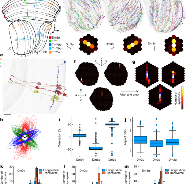
Supplementary Data 2 shows the locations of hexel types in coordinates. Following the convention defined in ref. 29, all three cardinal axes of the hexagonal lattice point upwards (Fig. 1f). The vertical axis is directed dorsally. The p and q axes are located inside the medulla, where they’re directed in two directions. The top and bottom of the hexagons are flat, while the left and right sides of the lattice have a scuplture. Due to the medulla being curved, the relation of the p–q axes to the dorsoventral and antroposterior axes is more complex.
The figures portray the lattice of medulla columns. A lattice similar to the lattice of medulla columns can be constructed for ommatidia, and this lattice is left–right inverted. The motion on the medulla lattice is front-to-back. In other words, the p and q axes are swapped in the eye relative to the medulla. Another difference between the eye and the medulla is that the p and q axes are close to orthogonal in the medulla, which is squashed along the anterior–posterior direction. The p and q axes are closer to 120° apart in the eye, where the ommatidia more closely approximate a regular hexagonal lattice.
Discriminating 2D projections with both intrinsic and boundary types by running from the 1 to the N points of a hexagonal lattice
Suppose that I run from the 1 to the N points of a hexagonal lattice when I see an image with hexel values. Normalizing the image yields a probability distribution ({p}{i}={h}{i}/({\sum }{j=1}^{N}{h}{j})). Then compute the coordinates of the image centroid by
mathopsum limits_i=1Np_i
We discovered that it was sufficient for feature dimensions to have only intrinsic types. Alternatively, feature dimensions can be defined as including both intrinsic and boundary types (T > 700), and this yields similar results (data not shown).
The sums are in the brain. The Wst/Ds+, which is the output fractions of type s, can be normalized by degree and run from 1 to T. The input fractions of type t are similar to the input fractions of type Wst/Dt.
The input and output feature vectors can be normalized by degree to yield input and output fractions of cell i, Oit/di+ and Iti/di−. Elements of these matrices are used for the discriminating 2D projections (Extended Data Fig. 3c.
Discriminators for all types in all families containing more than one type are provided in Supplementary Data 4. Many although not all discriminations are highly accurate. Both intrinsic and boundary types are included as discriminative features.
We can see all cells in the Pm family in two dimensions, by using the C3 input fraction and TmY3 output fraction. In this space, Pm04 cells are well-separated from other Pm cells, and can be discriminated with 100% accuracy by ‘C3 input fraction greater than 0.01 and TmY3 output fraction greater than 0.01’. This conjunction of two features is a more accurate discriminator than either feature by itself.
Finding the nearest logical predicates for a given type of cell: I. Searching for the simplest and most accurate tuples
The drop in the quality of the predicates if there is only one type is measured. As is the case with the clustering metrics, the impact on predicates is marginal (weighted mean F-score drops from 0.93 to 0.92).
On a high level, the process for computing the predicates is exhaustive—for each type, we look for all possible combinations of input type tuples and output type tuples and compute their precision, recall and F-score. A few optimization techniques are used to speed up this computation, by calculating minimum precision and recall thresholds from the current best candidate predicate and pruning many tuples early.
Because the feature vector is rather high dimensional, it would be helpful to have simpler insights into what makes a type. A method of finding a set of simple logical predicates is based on the link between the type and accuracy. For a given cell, we define the attribute ‘is connected to input type t’ as meaning that the cell receives at least one connection from some cell of type t. Similarly, the attribute ‘is connected to output type t’ means that the cell makes at least one connection onto some cell of type t.
True positive predictions are counted in the ratio of true positives to the total number of positive predictions.
We estimated the centre of each type using a trimmed mean after we arrived at the final list. Then, for every cell, we computed the nearest type centre by Jaccard distance. For 98% of the cells, the nearest type centre was near the assigned type. We sampled some disagreements and reviewed them manually. In the majority of cases, the algorithm was correct, and the human annotators had made errors, usually of inattention. The remaining cases were mostly attributable to proofreading errors. There were also cases in which type centres had been contaminated by human-misassigned cells (see the ‘Morphological variation’ section), which in turn led to more misassignment by the algorithm. After addressing these issues, we applied the automatic corrections to all but 0.1% of cells, which were rejected using distance thresholds.
Programmatic tools were created to help with searching for cells of the same type. One important script traced partners-of-partners, that is, source cell downstream partners or source cellupstream partners. This was based on the assumption that cells of the same type will probably synapse with the same target cells, which often turned out to be true. The tool could either look for partners-of-all-partners or partners-of-any-partners. The result was a long list of cells and was sorted by cells that had already been identified, or segments with small sizes or low ID numbers. Definition of layers was aided by a tool created from tangential cells of the lobula plate. This facilitated identification of various cell types, especially T4 and T5.
Citizen scientists created farms in FlyWire or Neuroglancer with all the found cells of a given type visible. There was a display of where cells still remained to be found. If they found a bald spot, a popular method to find missing cells was to move the 2D plane in that place and add segments to the farm one after another in search of cells of the correct type. Farms also helped with identifying cells near to the edges of neuropils, where neurons are usually deformed. Having a view of all other cells of the same type made it possible to extrapolate to how a cell at the edge should look.
Citizen scientists created a comprehensive guide with text and screenshots that expanded on the visual guide. They also found and studied any publicly available scientific literature or resources regarding the optic lobe. They shared findings at discuss.flywire.ai, which as of 10 October 2023 had over 2,500 posts. Community managers interacted with citizen scientists by sharing findings from the scientific literature, consulting Drosophila specialists on FlyWire and providing feedback.
Additional community resources foster an environment for sharing ideas and information between members of the community. Community managers answered questions and provided resources, such as a visual guide and shared updates. Each day’s daily statistics, including the number of annotations submitted, were shared on the discussion board. Live interaction, demonstrations and problem solving took place during the weekly video livestreams from the community manager. The environment created by these resources allowed citizen scientists to self-organize in several ways: community driven information sharing, programmatic tools and ‘farms’.
Source: Neuronal parts list and wiring diagram for a visual system
A connectomic cell approach to morphological cell typing: a case for missing synapses in the optic lobes
The optic lobes are divided into five regions (neuropils): lamina of the compound eye (LA); medulla (ME); accessory medulla (AME); lobula (LO); lobula plate (LOP). All non-photoreceptor cells with synapses in these regions are split into two groups: optic lobe intrinsic neurons and boundary neurons.
The top 100 players had been invited to make sure their work was perfect. They were made to label their neurons when they felt confident after three months of having their brains checked. Most citizen scientists do a mix of both. Sometimes they looked for cells of a specific type to look for after making sure they’re all right.
Our connectomic cell approach to typing is initially seeded with some set of types, to define the feature vectors for cells (Fig. 2a), after which the types are refined by computational methods. For the initial seeding, we relied on the time-honoured approach of morphological cell typing, sometimes assisted by computational tools that analysed connectivity. It is worth noting that ‘morphology’ is a misnomer, because it refers to shape only, strictly speaking. Orientation and position are actually more fundamental properties because of their influence on stratification in neuropil layers. Thus, ‘single-cell anatomy’ would be more accurate than morphology, although the latter is the standard term.
Finally, it may be known from other studies that a connection does not exist. T1 cells lack output. In our analyses, we discarded the few T1 synapses that were left because we thought they were false positives.
Extreme asymmetry is one of the reasons to look for it. If the number of A to B connections is larger than that of B to A, the connection might be spurious. The huge contact area between A and B is the reason for the high false- positive rates.
In the central brain, most cell types have cardinality 2 (cell and its mirror twin in the opposite hemisphere; Extended Data Fig. 1e). The hemibrain has one cardinality. Since most of the connectomic data is not yet available, there are only two or three examples of the ordered pair that can be used to decide whether there is a connection between cell types A and B. If false positives can be avoided, setting the threshold to a relatively high value is a good idea.
The seven column reconstruction provided a matrix of connections. The agreement shown with the data shows a check on accuracy of the reconstruction. This validation complements the estimates of reconstruction accuracy in the central brain that are provided in the flagship paper24.
The seven column reconstruction says that Tm21, Dm2, TmY5a, Tm27, and Mi15 are not modular. On the other hand, some of our types (T2a, Tm3, T4c and T3) contain more than 800 proofread cells (Fig. 1d), which violates the definition of modularity. This partially agrees with the seven column reconstruction28, which regarded T3 and T2a as modular, and T4 and Tm3 as not modular. T4 is an unusual case as it is above the other T4 types. It should be noted that all of the above cell numbers could still creep upward with further proofreading.
The Logarithmic Fragmentation of the Intrinsic Volume of our Cells. I. The Photoreceptors in the FlyWire Connectome
The brain volume of the 84% of our cells that are intrinsic to it. The central brain and the optic lobes have the same number of neurones. inputs and outputs in the central brain are stored in visual projection neurons. Visual centrifugal neurons have inputs in the central brain and outputs in the optic lobe. The brains are divided into classes based on sensory neurons entering the brain from the periphery. If you need more information on the classification criteria, refer to our companion paper. We used some labels contributed by the FlyWire community.
The inner photoreceptors R7 and R8 are about 650 cells each, and the outer photoreceptors R1–6 total about 3,400 in version 783 of the FlyWire connectome. These numbers are not inconsistent with modularity because photoreceptors are especially challenging to proofread in this dataset and under-recovery is higher than typical.
left, left, left, left
and the weighted Jaccard distance d(x,y) is defined as one minus the weighted Jaccard similarity. The quantities are all zero and one if you count the featurevectors that are non negative. In our cell typing efforts, we have found empirically that Jaccard similarity works better than cosine similarity when feature vectors are sparse.
This cost function is convex, as d is a metric satisfying the triangle inequality. The cost function has a minimum. We used various approximate methods to minimize the cost function.
Source: Neuronal parts list and wiring diagram for a visual system
Neuronal Parts List and Electrical Diagram for a Visual System: Auto-correction with the Trimmed Mean and Cytoscape81
The trimmed mean is used for auto-correction of type assignments. We found empirically that this gave good robustness to noise from false synapse detections. For the type radii, we used a coordinate descent approach, minimizing the cost function with respect to each ci in turn. The loop included every i for which some xi was non-zero. This happened within a small part of the loop.
The precise memberships in the clusters warrant cautious interpretation, as the clusters are the outcome of just one clustering algorithm (average linkage), and differ if another clustering algorithm is used. Each cluster has core groups of types that are similar to each other and that merge early during agglomeration. These are more certain to have similar visual functions, and tend to be grouped together by any clustering algorithm. The types that are merged late are less similar, and their cluster membership is more arbitrary. It’ll happen when one divides the visual system into seperate subsystems because subsystems that interact with each other are borderline cases.
We used Cytoscape81 to draw the wiring diagrams. Organic layout was used for Figs. 3 and 7c, and hierarchical layout was used for the others. The layout is meant to make arrows point downwards. After Cytoscape automatically generated a diagram, nodes were manually shifted by small displacements to minimize the number of obstructions.
Source: Neuronal parts list and wiring diagram for a visual system
The Class, Families and Types of Axons in the Visual Dendrites of the Neural Networks (in Supplementary Data 5)
There are at least 5% of the brain’s connections in the eyes and less than 5% in the other parts.
In the main text (in the ‘Class, family and type’ section), we used the term ‘axon’. Axon refers to a portion of the neuron that has a high ratio of pre and postsynapses. This ratio is very high in a sense. The ratio in the axon could be related to the others in the neuron. In either case, the axon is typically not a pure output element, but has some postsynapses as well as presynapses. For many types it is obvious whether there is an axon, but for a few types we have made judgement calls. The axon can be seen from the presence of pre-synaptic boutons, even without examining the sphinx. The opposite of an axon is a dendrite, which has a high ratio of postsynapses to presynapses.
There are four amacrine types that extend over the medulla and lobula. LMa1 to LMa4 are coupled with T2, T2a and T3, and LMa4 and LMa3 synapse onto T4 and T5 (Supplementary Data 5). The Amacrine cell that extends over both the lobula and medulla is said to be in the LMa family. However, the new LMa types consist of smaller cells that each cover a fraction of the visual field, whereas CT1 is a wide-field cell.
A local interneuron is defined as being completely confined to a single neuropil (Fig. 1b). The majority of types areneurons, while there are a minority of cells. There is only one interneuron in this area. Dm and Pm interneurons6 stratify in the distal or proximal medulla, respectively. More than doubled the number of Pm types and slightly increased the number of Dm types. The Sm family contains more types than any other family, and it’s almost completely new. The lobula plate is where the Li and the LPi interneurons are located. Interneurons are a mixture of amacrine and cholinergic. Interneurons are often wide field but some are narrow field.
After two lobula intrinsic types (Li1 and Li2) were initially defined6, 12 more (Li11 to 20 and mALC1 and mALC2) were identified by the hemibrain reconstruction9. We have confirmed the following: Li2, Li12, Li16, mALC1, and mALC2. We identified 21 additional Li types, but have not been able to make conclusive correspondences with previously identified types. As mentioned earlier, we transfer Tm23 and Tm246 from the Tm to the Li family. This amounts to a total of 33 Li types, which have been named Li01 to Li33 in order of increasing average cell volume.
Pm1, 1a and 26 are classified into two different types. Pm3 and 4 are the same as before. In order to increase the average cell volume, we identified six new Pm types with the number Pm01 to Pm14 written on them. The old names can be distinguished from the new ones with leading zeros. Predicted are the effects of giaergic. Pm1 was split into Pm06 and Pm04, Pm1a into Pm02 and Pm01, and Pm2 into Pm03 and Pm08.
Source: Neuronal parts list and wiring diagram for a visual system
LPi Types: Names of Large Recurrent Neurons based on Single Cell Anatomy, Ort Expression, and a New Family of Tangential Types
We discovered one tangential type that projected from the lobula to lobula plate, and called it LLPt. This is just a single type, rather than a family.
Now that LPi types have multiplied, stratification is no longer sufficient for naming. Adding letters to distinguish between cells of different sizes is how the naming system could be salvaged. For example, LPi15 and LPi05 could be called LPi2-1f and LPi2-1s, where ‘f’ means full-field and ‘s’ means small. For simplicity and brevity, we instead chose the names LPi01 to LPi15, in order of increasing average cell volume. The Codex documentation details the old stratification-based names in the letters.
We applied the following criteria to identify large recurrent neuropil-specific neurons. First, the neurons were intrinsic and met the rich-club criteria. At least fifty percent of the neuron’s incoming connections were contained within a single neuropil. Third, at least 50% of the neuron’s outgoing connections were contained within the same neuropil.
Single-cell anatomy and Ort expression were used to define Tm5a, Tm5b and Tm5c. Tm 5a is a cholinergic, the majority of the cells have at least one dendrite from M6 to M3. Tm5b is cholinergic, and most (~80%) cells extend several dendrites from M6 to M3. Tm5c is glutamatergic and extends its dendrites up to the surface of the distal medulla. Three types are in agreement with the description in fig. 7a and get input from inner photoreceptors R7 or R8.
There are subnetworks in which all cells can be reachable through directed pathways. The directionality of connections is not taken into account when evaluating WCCs in which all neuron are mutually reachable.
For a given neuron i, the in-degree ({d}{i}^{+}) is the number of incoming synaptic partners the neuron has and the out-degree ({d}{i}^{-}) is the number of outgoing synaptic partners the neuron has. Thetotal degree of a neuron is the sum of in- and out- degrees.
We compared the statistics of different null models with those of the wiring diagram G(V,E). The ER model we used is a directed version where all edges are drawn independently at random and connection probability is set so that the number of edges in the ER model equals. The connection probability is constant for any one of the following:
The (global) clustering coefficients shows the probability of three cells being connected, regardless of directionality.
The metrics were computed across the whole-brain and within-brain-region. We also systematically quantified the occurrence of distinct directed three-node motifs within the network, ensuring that duplicates are eliminated: any subgraph involving three unique nodes is counted only once in our analysis. To compute the expected prevalence of specific neurotransmitter motifs (Figs. 2c and 3d,e), we multiplied the relevant neurotransmitter probabilities for the motif of interest, under the assumption the neurons connect independent of neurotransmitter. The true frequencies of these neurotransmitter combinations were compared to this expectation.
As reciprocal edges in the wiring diagram are over-represented when compared to a standard ER model, we adopted a generalized ER model, which preserves the expected number of reciprocal edges. The ER model has two parameters, a type of connection probability puni and an inverse type of connection probability pbi. To do this, we defined the sets of unidirectional and bidirectional edges as:
The NPC model: A spatial null model based on a modified version of the Maslov-Sneppen model developed by switching-and-hold
In Ewedge it is used for the beginning of thearray and the end of it. (j,i)\notin E},\ {E}^{{\rm{bi}}}\,:= \,{(i,j){\rm{| }}(i,j)\in E\wedge (j,i)\in E}.\end{array}$$
$$\begin{array}{l}P\left[{i}{\nleftarrow }^{\to }\,j\right]=P\left[{i}{ \nrightarrow }^{\leftarrow }\,j\right]={p}^{{\rm{uni}}}=\frac{\left|{E}^{{\rm{uni}}}\right|}{\left|V\right|\left(\left|V\right|-1\right)},\ P\left[{i}{\to }^{\leftarrow }\,j\right]={p}^{{\rm{bi}}}=\frac{\left|{E}^{{\rm{bi}}}\right|}{\left|V\right|\left(\left|V\right|-1\right)},\ \left[{i}{ \nrightarrow }^{\nleftarrow }\,j\right]=1-2{p}^{{\rm{uni}}}-{p}^{{\rm{bi}}}.\end{array}$$
The directed configuration model is the same one that we used in previous work. We used the switch-and- hold variant to randomly select two edges in each iteration and swap their target endpoints, or alternatively, we kept them the same. This models is equivalent to the null Maslov–Sneppen model 66,67,68.
To provide a more tractable spatial null model while preserving degree sequences, we developed the NPC model. There is a degree-corrected stochastic block model. We assigned each neuron to one of the 78 ‘neuropil blocks’ based on the neuropil in which the neuron has the most outgoing synapses. During random rewiring, the inter- and intra-neuropil connection probabilities are preserved. We keep the degree sequence the same during randomization while prohibiting self-loops and multiple edges. The interneuropil connection densities contain information about the world around them. These constraints also mean that the total number of internal edges in each neuropil remains the same after reshuffling.
where (\Pi := {\rm{Diag}}({\rm{\pi }})) and I is the identity matrix. We defined (mathcalLrmrev) as the reverse Markov chain. The eigen-spectra of ({\mathcal{L}}) and ({{\mathcal{L}}}^{{\rm{rev}}}) are shown in Extended Data Fig. 1f,g, respectively. The gaps between eigenvalues indicate the conductance properties of the graph.
Pi is a part of the equation.
Source: Network statistics of the whole-brain connectome of Drosophila
A small-worldness study of the rich-club connectome in the whole-brain fly and integrator neurons in the CFG null model
There is a number of connections between the neurons in the network with degree d and Md. To control for the fact that high-degree nodes have a higher probability of connecting to each other by chance, we normalized the rich club coefficient to the average rich club value of 100 samples from a CFG null model (Fig. 1h and Extended Data Fig. 2e,f):
The standard method of determining the rich-club threshold is to look for values of k for which Φnorm(d) > 1 + nσ, where σ is the s.d. of ΦCFG(d) and n is chosen arbitrarily20. The start threshold of the rich club was defined as norm(d) > 1.01 due to the very small sample size.
To find out the small-worldness of the connectome we compared it to an ER graph. The average undirected path length in the ER graph, denoted as ({{\ell }}{{\rm{rand}}}), is estimated to be 3.57 hops, similar to the observed average path length in the fly brain’s WCC (({{\ell }}{{\rm{obs}}}=3.91)). The ER graph’s clustering coefficients are smaller than the observed ones. (Table 2). The whole-brain fly connectome has a small-worldness coefficients.
Similarly, we identified integrator neurons by filtering the intrinsic rich-club neurons for those that had an in-degree that was at least five times higher than their out-degree:
The model we ran used different subsets of sensory cells as seeds, such as olfactory, gustatory, and mechanosensory cells. We also ran the model using the set of all of the input neurons as seed neurons. All neurons in the brain were then ranked by their traversal distance from each set of starting neurons, and this ranking was normalized to return a percentile rank. We say that the visual projection neurons are a proxy for visual inputs to the central brain.