A 3D-printed syringe-based system for dynamic interface printing using a high resolution, low-resolution optical projection module
Dynamic interface printing, a process that the authors of the article refer to and over which they claim several advantages, is an invention of H.T. H.T. carries out research, holds funding related to CAL, and holds several patents on CAL and a small number of shares in a company that holds a licence to practice CAL.
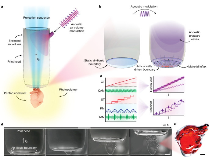
New approaches to 3D printing promise to transform how objects are produced to serve a broad range of industries. Digital light manufacturing is, in part, a category of 3D-printing processes that uses patterns of light projected onto a liquid to cause the liquid to solidify at a defined position. The ultimate goal is to develop these processes to rapidly print features at microscopic scales using a range of materials, with excellent surface finishes and at sizes suitable for industrial applications (potentially up to a scale of many centimetres). The quality of the resulting objects is reduced due to light patterns in the liquid and practical issues that limit the speeds of current processes. Writing in Nature, Vidler and colleagues1 report a 3D-printing strategy that could solve these problems.
The components of the system were mounted on the optical breadboards to make sure they were perfect. 2a). The images were captured using a high-power projection module with a resolution of 2,560 1,600 and a size of 15.1 m. The projection module and print head were positioned in the z direction using a 100 mm linear stage (MOX-02-100, Optics Focus) affixed to the vertical breadboard. The position of the air–liquid interface was controlled by a 50 ml syringe connected to the print head with a silicone tube and pressurized using a 50 mm linear stage (MOX-02-50, Optics Focus). Two further linear stages enabled location of the well plate for sequential or multi-step printing. The motion control was managed using a commercially available 3D printer control board. The 4k camera and 16mm lens was used to record the printing process.
A second system iteration was developed for in situ imaging, with modifications to allow the printing container to move relative to a stationary probe (Supplementary Fig. 3). The system incorporated a custom CoreXY motion system and a NEMA 23 ball-screw linear stage to translate the entire CoreXY stage relative to the stationary print head. The blue mirrored dichroic mirror and a 50:50 beamsplitter were used to illuminate in situ. The illumination was either provided with or without a custom well-plate holder. To maintain physiological temperatures and sterility during printing, the motion components and print head were enclosed within a custom heated chamber. Sterility was maintained by continuous HEPA filtration during printing, surface sanitization with 70% ethanol and sterilization with UV-C before use.
Acoustic modulation of the air–liquid interface was achieved by direct volume manipulation of the air volume within the print head. The approach was simple. The set-up consisted of a 3 inch 15 W voice coil driver (Techbrands, AS3034) affixed to an enclosed 3D printed manifold containing an inlet and outlet port (Fig. 3a and Supplementary Information section 2 and Supplementary Fig. 1c,d). The voice coil was driven by a commercially available amplifier (Adafruit, MAX9744) using the supplied auxiliary port, with specified waveforms sent by the MATLAB GUI. The frequency ranged between 1 and 500 Hz when possible, with fixed or transient frequency or amplitude switching. By specifying a waveform for each degree of freedom it was easier to align the acoustic modulation with all the motion, optical and pressure control.
The synthesis of Norbornene-functionalized sodium alginate by dissolving PEGDA Mn 700 (455008, Sigma) in a mixture of tartrazine and LAP
We followed a same protocol for all of the different concentrations used in the study. The required weight fraction of PEGDA Mn 700 (455008, Sigma) was dissolved in the corresponding volume fraction of 40 °C deionized water (excluding 100% w/v) and thoroughly mixed for 10 min. Subsequently, 0.035 w/w% of tartrazine (T0388, Sigma) and 0.25% w/w of LAP (900889, Sigma) were added to the mixture and stirred until complete dissolution. TheFalcon tubes were used to store the materials until required.
Warming the mixture to 40 C and then stirring it resulted in a solution of 500 IU of phenylbis(2,4,6-trimethylbenzoyl) phosphine oxide. To control the resolution in the z direction, the photo-absorber Sudan I (103624, Sigma) was added in various quantities ranging from 0 to 0.04% w/w. Falcon tubes were used to store the materials until required.
The substitution rate of GelMA was confirmed by a nuclear magnetic resonance. A 10% w/v GelMA solution was prepared by dissolving 1 g of GelMA in 10 liters of cell culture media. When complete dissolution of GelMA was achieved, 3.5 Mg of tartrazine and 25 grams of LAP were added to the solution. The mixture was sterilized by passing it through a 0.22 µm sterile filter within a biosafety cabinet and subsequently stored in refrigerated light-safe Falcon tubes until required.
A previously reported protocol57 was the basis of the synthesis of Norbornene-functionalized sodium alginate. In short, 10 g of sodium alginate were dissolved in 500 ml of 0.1 M 2-(N-morpholino) ethane-sulfonic acid buffer (145224-94-8, Research Organics) and fixed to pH 5.0. There was an addition of over 10 g of 1-ethyl-2-(3-dimethyl-9-yl) Carbodiimide•HCl, 2.90 g of N-hydroxysuccinimide, and over 3 lbs of 5-norbornene-2-methylamine. The pH was fixed at 7.5 with 1 M NaOH. The reaction was carried out at room temperature for 20 h. The mixture was dialysed against water for 5 d before lyophilization. The degree of functionalization was determined by the 1H nuclear magnetic resonance. A 7 percent w/v sodium calcium solution was prepared by dissolving 1 g of the salt in 14.29 liters of thebuffered saline solution. Next, 5 mg of tartrazine, 36 mg of LAP and 122.7 µl of 2,2′-(ethylenedioxy)diethanethiol were dissolved in 5.59 ml of phosphate-buffered saline, added to the sodium alginate solution and mixed until it was homogeneous. The pH was adjusted with 1 M NaOH until the solution was visibly opaque.
A solution of 50 mg of phenylbis(2,4,6-trimethylbenzoyl) phosphine oxide (511447, Sigma) and 5 g of diurethane dimethacrylate (436909, Sigma) was prepared by warming the mixture to 45 °C and stirring for 30 min. To remove residual air bubbles after 10 minutes, the mixture was transferred to a light-safe Falcon tube andcentrifugationd at 4,000rpm.
Source: Dynamic interface printing
Preliminary Determination of Human Renal Cell Viability in a DIP 3D Printing System Using Thingiverse.com
Human embryonic kidney 293-F cells (Freestyle 293-F, Thermo Fisher) were used in a preliminary determination of the cell viability of the DIP 3D printing system. In this work, a cell solution with 7.2 million cells per millilitre was used for both the model of the kidney and the cell-viability measurements. To determine cell viability a thin 500 m wall was printed to minimize the effect of cell death due to insufficient media dispersal, which was imaged using a live/dead viability/toxicity kit. Three structures were printed (n = 3), and measurements were taken after 24 h to determine the preliminary viability of the technique. Cell viability was determined at three locations for each sample (s = 3), with the total viability being an average of all collection points (Supplementary Fig. 18).
Three-dimensional design models of Bowman’s capsule, a tri-helix structure and a Kelvin cell were created using nTop. The models were downloaded from Thingiverse.com. The files were sliced using Chitubox and then put into a stack of images. The frame rate of the signal was limited to 120 frames per second, so we often used projection frame rates that matched the acoustic driving frequencies to minimize motion blur. The object was moved into a voxel array based on the desired print speed and frame rate. The layer height (Lh) was determined as ({L}{{\rm{h}}}={v}{z}/f), where vz is the linear print speed and f is the acoustic excitation frequency, which matched the projection frequency. The image stack was further corrected in order to create a secondary image stack, which was sent to the projector over HDMI using PSYCHtoolbox-2. The print sequence started by moving the print head to a defined distance above the print surface (or high-density material). When the interface was brought with the image plane contingent on the chosen print head, it automatically brought coplanar with it. The MATLAB GUI was operated by first sending a signal to turn on the LED module and subsequently controlling the location of the air–liquid interface by modulating the pressure, acoustic driving and translation location. The optical power of the projection module could be adjusted using the space matrix. For prints made with HDDA, the printed structures were removed from the print volume and washed with isopropyl alcohol. If you made structures from GelMA or PEGDA, the excess material was gently removed using a pipette and resuspended in deionized water or cell culture media. If required, the structures were fluidically detached from the bottom of the container and stored in an appropriate solution.
The curved surface used in this work differs in geometric discretization from a traditional flat construction surface. A detailed explanation of the convex-slicing process is given in the Supplementary Information. However, the main components will be briefly restated here. First, the general shape of the interface was determined by the Young–Laplace equation, (\Delta p=-\,\gamma \nabla \cdot \widehat{n}), which describes the Laplace pressure difference ((\Delta p)) sustained across a gas–liquid boundary dependent on the material surface tension ((\gamma )) and surface normal ((\hat{n})). Here, we used axisymmetric print containers such that (\hat{n}) can easily be found by substituting the general expressions for principal curvatures. The longest capillary length used was rho g, where is the material surface tension and is the material density. The result was an ordinary differential equation for the interface shape.
This equation can be readily solved using numerical integration with appropriate boundary conditions (Supplementary Information section 4). However, using this method would require numerical integration for the steady-state case, and moreover, we would need to solve each intermediate state during compression with the associated boundary conditions. We, instead, opted to approximate the solution using cubic Bézier curves for the steady-state case and approximating the compressed profiles by geometrically deforming the Bézier curve while ensuring volume equivalency (Supplementary Information section 7). This is faster since there are a lot of intermediate surfaces in the Transient region. The half-profile was revolved around the central z axis in order to convert the 2D Bézier solution into a 3D surface. The surfaces were starting at the compressed state and transitioning to the interface profile. The projection of the voxel grid and surface array was determined by the distances between them. Reconstruction accuracy was validated by ‘replaying’ the projections over an empty voxel array and computing the Jaccard index between the reconstructed voxel array and the input voxel array (Supplementary Information sections 8 and 9).
We used a similar approach to determine our theoretical optical model, which was done by Behroodi et al.59. To determine the effective energy delivery and depth of cure, a ray incident on the meniscus was decomposed into reflective and transmissive components, described by a transmissive efficiency. The irrerly index of the air and liquid is represented by n1 and n2 and the normal point on the meniscus is (hatbfu). The energy intensity was calculated as a Beer–Lambert decay. As the interface is curved, the effective resolution is spatially dependent on the local height of the meniscus relative to the focal plane. We mapped the coordinates of the focal plane to that of the meniscus surface, creating a large map of the effective size across the interface. This map was used to estimate the area fraction based on the print head’s size and material properties.
To understand the formation of acoustically driven capillary-gravity waves, we used many established analytical approaches that describe the induced velocity and secondary streaming effects32 created by the meniscus (Supplementary Information sections 13–15). This analysis establishes the velocity scaling laws of capillary-gravity waves dependent on the effects of capillary or gravity. The dispersion relation is related to the wave number and the wave frequencies. We, therefore, show that ({(\lambda /{l}_{{\rm{cap}}})}^{2}) is a unitless quantity that relates the dominance of surface tension and acoustic parameters on the flow magnitude (Supplementary Information section 14). The capillary length of the material is marked by lcap. As U, the flow velocity scales as lambda MU, for example. Supplementary Fig. 19 shows the effect of material and acoustic parameters on velocity scaling.
The 3D flow field was produced below the air–liquid boundary by PIV. A high-speed camera (Kron Technologies, Chronos 1.4 Camera) was used to capture footage of 20–50 µm poly(methyl methacrylate) Particles, both normal and outlier, go to the air–liquid boundary. Particle tracing and velocity reconstruction were performed on the captured video sequences using PIVLab (ref. 60) for MATLAB. The exact parameters and methodology used can be found in Supplementary Information section 18. The velocity profiles for top-down and side are shown in Fig. 3c–e and Supplementary Figs. 8 and 9.
To determine the transient interface restabilization in the bulk flow, high-speed photography under a uniform backlight was captured at 5,000 fps (Supplementary Fig. 7). Restablization was determined by segmenting the center line and recording the video’s yap in real time. The interface settling time was determined by applying an exponential criterion set at 1/e2 of the starting amplitude.
The material influx rate with and without acoustic excitation was determined by filling a glass cuvette with materials doped with black dye to prevent light transmission. The cuvette was placed on top of a red backlight, such that when the air–liquid boundary formed against the base of the cuvette, the transmitted light was observed by a CCD (Supplementary Information section 19). The material influx rate was measured by raising the air–liquid boundary with and without acoustic excitation and tracking the influx of dyed material, which occluded the backlight transmission (Fig. 3f and Supplementary Information section 20 and Supplementary Fig. 11).
Source: Dynamic interface printing
Micro computed tomography using a Phoenix Nanotom M scanner, X-ray scanning electron microscope and helium ion microscopy
Micro computed tomography images were acquired using a Phoenix Nanotom M scanner (Waygate Technologies, voxel size of 10 µm3, 90 kV tube voltage, 200 µA tube current and 8 min scan time). Tissue paper was mounted into a tube to hold the samples for X-ray. For hard materials such as HDDA, the structures were placed on a plastic cap to provide good contrast between the printed structure and the supporting medium. Keyshot 11 imported an STL surface mesh to make a final micro computed tomography representation.
Fluorescence microscopy images were captured using a Zeiss Axio Observer Z1 (Zeiss) using either a ×4 or a ×10 objective. For constructs that were larger than the objective’s field of view, the images were stitched together in the software to create a large format image. Once the fluorescence images were acquired, cell-counting was performed on each live/dead image pair using a custom MATLAB script.
The FlexSEM 1000 is a scanning electron microscope. Printed structures on glass slides were mounted directly on the microscope stage with no further sample preparation. The samples had no coating on them. The electron microscope was operated in variable-pressure mode at 50 Pa. Images were acquired with a 15 keV beam using the ultra-variable detector. To cover the field of view needed for the large structures, the working distance was typically 40–50 mm, and several images were collected in a tiled manner and stitched together in postprocessing.
Helium-ion microscopy images were acquired with a Zeiss NanoFab using a helium source. During imaging, the flood gun was used to actively neutralize the surface, thus removing the need for a conductive coating. The structures were imaged using a current of 1 to 2 pA, and a field of view of 1,100 m. The structures were printed on the slide and mounted using the clips on the stage. A number of images were taken and then stitched together using imageJ/ fiji to facilitate the capture of larger structures.