Clustering and analysis of human stem cell samples from the SpatialLIBD Project: application to the brain Visium data from late-stage tumours
The human GBM stem cell dataset (20 samples) from ref. 53 was downloaded from the Single Cell Data Portal and analysed using the same analysis pipeline and parameters as for our tumorigenesis atlas dataset except with human orthologues. The same quality control cutoffs as for our atlas were used; Seurat and Harmony were used to integrate, correct batch effects, and cluster cells together. The same computational pipelines as for our atlas were used for computing the top differentially expressed genes and inferring CNAs.
For the human Visium samples, which consist of late-stage tumours with almost no normal regions, we turned to the normal brain Visium data from the SpatialLIBD Project. We randomly selected two slides from the project as references and conducted inferCNV for each, to make sure there were no reference biases. Both references yielded congruent outcomes.
We recognized the importance of the reference data to ensuring result accuracy, and chose it with care. The normal regions within each slide were used for the mouse Visium. We clustered spots on the basis of their RNA profiles. Among the RNA clusters corresponding to normal regions, we earmarked one as the reference and set aside the remaining normal clusters as negative controls. Our analysis using inferCNV revealed no distinct CNVs in these normal region clusters, whereas tumour regions exhibited pronounced CNVs.
We used Seurat’s subset function to isolate the malignant cells, which belong to the Sox2CEPPT and nestinCPPT mouse model samples, from the main atlas. The following parameters were used to recluster these malignant cells: data normalization was performed with the LogNormalize method and a scale factor of 10,000; a default value of 2,000 variable features with the vst selection method was used to determine the top variable features; data scaling was performed with regression of mitochondrial percentages. We used the new version ofHarmony to generate the embedded space for analysis. The closest neighbouring cells were identified using the rann method. We then annotated the cells using known cell type markers from the literature and differentially expressed genes.
The one-sided Fisher’s exact tests of the proportions of the cell types in different times were computed using the R package rstatix. For each time point, we calculated the number of cells in each cell category to construct the contingency table. The fisher test was used to perform the statistical tests.
The same computational pipeline and method as for the tumorigenesis atlas were used to remove doublets, and integrate and annotate the ten injury samples (Supplementary Fig. 9a). The following cutoffs were used to remove low-quality cells: percentage of mitochondrial >12%; number of genes detected per cell <800; number of UMIs per cell <500. We isolated the microglia and OL cells in separate analyses and recomputed their top differentially expressed markers separately. The abundance fractions of the different cell types in the relevant category of cell types (for example, PC types) in each time point were calculated as the number of cells for each cell type over the total number of cells from all the cell types belonging to that category in each time point, respectively.
The global relatedness between cell types was visualized with constellation plots, which we had implemented previously3,20. To generate the constellation plot, each transcriptomic cluster was represented by a node (circle), whose surface area reflected the number of cells within the subclass in log10 scale. The position of each node was based on the centroid position of the corresponding cluster in UMAP coordinates. The relationships between the two groups were indicated by the edges. For each cell, 15 nearest neighbours in reduced dimension space were determined and summarized by cluster. We separated the neighbours that were assigned to other clusters by the fraction. At the edges, at least one of the nodes had a higher percentage of nearest neighbours than the connecting one. The width of the edge at the node reflected the fraction of nearest neighbours that were assigned to the connecting node and was scaled to node size. For all nodes in the plot, we then determined the maximum fraction of ‘outside’ neighbours and set this as edge width that was 100% of node width. The function for creating these plots, plot_constellation included in the R package scrattch.bigcat.
We evaluated the reconstructed cell phylogenies from two perspectives: clone identification and directionality of evolution. We used MEDALT and Hierarchical clustering to find the correct distance measures of the two different types of distances on the tree. MED was calculated using a method that is called MEDALT. The tree was loaded into R as an Igraph object and visualized using GGALLY, ggnet2 and igraph.
The CNAs in a cell are acquired in two ways: inherited from its parent cell; newly acquired during cell division. The whole tree we generated has a simulation of the entire sequence of events. We assume that each of the cells have a number of newly acquired CNAs. This means that with probability e−λ, a cell will not get any new CNA. was set between 0.25 and 0.6. CNAs can affect contiguous sites and regions in a chromosome, meaning that a gain (or loss) of copy for adjacent genes can happen together. We assumed the starting position of each CNA was uniformly distributed across the genome, and that there was a mean of 100–200 genes that one CNA affected in our simulation. The cells were selected for downstream analysis after each simulation.
To determine the relative abundance of individual cells like NSC-, NPC-, MSC-, and AC-. We put the total number of cells from all of the states together. The total number of cells in a time point was calculated as the number of cells for each cell state, divided by the fraction of each state. Further, to compare the relative abundances of the cell population categories across the four stages of tumour development, we first combined all of the non-cycling PC-like states (NSC-like, NPC-like, OPC-like and MSC-like) and designated them as non-cycling lineage PC-like. The differentiated states were combined and designated as differentiated-like. The third and fourth groups were the cycling PC-like and NCC-like cells. The fractions of four populations in each of the tumour samples were computed. The fractions were grouped based on the stages of the tumors. We plotted the averages along with their standard errors for each of the categories with respect to the four tumour stages (Extended Data Fig. 2a).
in which N0 is the initial number of cells, and b and d are the birth and death rate, respectively. The interval of time Δt between two adjacent events (the length of the branch in the phylogenetic tree) follows an exponential distribution with mean E(Δt) = 1/(b + d). When branching happens, it can be a birth with a probability of b/(b + d), or a death with a probability d/(b + d). The birth and death rates don’t change during the evolution according to our simulation.
Cell-cell communication analysis of tumors using R packages phateR, slingshot, and PAGA: A comparative study
The analysis of cell–cell communication was performed in chronological order for each of the four stages of tumors. We followed the official workflows with default parameters. First, we loaded the normalized counts into CellChat, followed by the preprocessing steps identifyOverExpressedGenes() and identifyOverExpressedInteractions(). We smoothed gene expression by applying a diffusion process on the protein–protein interaction network implemented in projectData() function. We then ran the computeCommunProb() function for communication analysis with the parameter population.size = FALSE to eliminate possible bias due to cell population size. This resulted in a network of communication strength between all cell states for each of the ligand–receptor pairs that passed the filtering steps. The communication strength of cell states at pathway and global levels was determined by the use of aggregation functions. For each of the pathways (data slot netP), we evaluated the role of different cell states as senders or receivers on the basis of the out-degree or in-degree of the communication network, implemented in the netAnalysis_signallingRole() function.
The R packages phateR v1.0.765 and slingshot v1.8.066 were used to build trajectories. First, we used phateR to generate two-dimensional (2D) embeddings (PHATE space), with the 50 harmony embeddings as input. The spanning tree of different cell types was built using a slingshot. For differential analysis, we first clustered cells into five clusters along the trajectory, and then the cluster-specific maker genes were found using the FinderAllMarkers() function in Seurat. To test the results, we used the diffusion map implemented in the R package to generate 2D embeddings of 50 harmony embeddings, as well as using PAGA to summarize the k-nearest neighbours. There were several methods that resulted in similar topologies between cell states.
Source: Gliomagenesis mimics an injury response orchestrated by neural crest-like cells
Genomics studies of mouse brain injury: characterization of glioma- and control mice using FACS cell sorting and 10x Genomics data transposition
This study used the mice from Jackson Laboratories, there were two exceptions. The glioma and control mouse models were generated and housed in 12-h dark–light cycle facilities maintained at appropriate temperature and humidity and in which mice had free access to water and chow. The mice were monitored and euthanized when they developed symptoms such as raised intracranial pressure. The ethical and legal regulations were followed in all of the mouse experiments. The animal use protocols were approved by the Animal Care Committees in the different institutions at the University of Toronto.
MRI was performed as reported previously8, and fresh brain tissue was collected from mutant mice at four MRI-defined stages: the ‘preneoplastic’ stage, at which the brain imaging shows no signs of neoplastic lesion development; the ‘early-lesion’ stage, characterized by small abnormalities seen on T2-FLAIR MRI sequences; the ‘mid-lesion’ stage, when the lesion has reached a larger size, as indicated by a T2-FLAIR-bright mass, in asymptomatic animals and occupies a substantial fraction of the brain hemisphere; and, finally, the ‘end-point’ stage, when mice develop symptoms of raised intracranial pressure or focal neurological abnormalities, with the tumour extending over a large portion of the brain hemisphere(s), typically with midline shift. Each brain tissue sample was dissociated into single cells as described previously8. FACS separated the live tTomatod+ cells and the tTomatod cells. Following sorting, both populations were characterized by scRNA-seq using the 10x Genomics platform as reported previously8. Tissue processing was performed in the same way for the Sox2eGFP mouse brain injury samples and was followed by cell sorting to separate the live GFP+ and GFP− cells. For scATAC-seq, the nuclei were isolated from sorted cells and processed using the 10x Genomics Single Cell ATAC-seq workflow and following the manufacturer’s protocol (user guide CG000168 Rev A). In brief, 5 μl of nucleic suspension was added to the transposition reaction, which was used for the gel beads-in-emulsion (GEMs) generation and barcoding on the 10x Chromium Chip E for PCR amplification. DNA was recovered using Dynabeads MyOne Silane beads, which proceeded to library preparation to add Chromium i7 Sample Index N Set A library barcodes. To check for size on the 800 bioanalyzer, libraries were checked for quantifiably by using the kabuki library quantification protocol. Illumina recommended a protocol for generating 50 base reads from the libraries pooled in equimolar quantities on the Illumina Novaseq platform. Spatial transcriptomics was performed on formalin-fixed and paraffin-embedded mouse tissue sections using the 10x Genomics Visium platform and following the manufacturer’s protocols (user guides CG000407 Rev D and CG000409 Rev C).
The mice were ready to go for surgery. The incel Cannula was implanted at 1.5mm to the left and the osmotic pump was put in following the manufacturer’s instructions. Each osmotic pump was filled with normal saline to infuse the brain at a flow rate of 0.5 µl h−1 for 5 consecutive days.
Removing off-target cells from downstream analysis of scRNA-seq data from the ABC-WMB atlas
To assure that downstream analysis is not biased by the integration method, we used FastMNN60, implemented in SeuratWrappers, to redo the batch correction. These methods all gave similar results (Supplementary Fig. 6).
We first isolated the PC- like cells and then removed all of the genes from the cell cycle mouse orthologues which were linked to the S and G2/M phases. The 205 cell cycle genes needed to be removed to hide the high levels of their genes that are associated with cycling. Reclustering revealed that there are six cycling cells: NSC-, OPC-,NPC-, MSC-, and AC-. To compute the fractions of cycling and non-cycling cells for each of the precursor-like malignant states (NSC, OPC, NPC, MSC and NCC), we calculated the number of cycling and non-cycling cells for each precursor state in each of the samples. The fractions of cycling and non-cycling cells for each PC-like state were calculated as the number of cells over the sum of both cycling and non-cycling cells. We plotted the averages with their standard errors.
Each sample was processed in Seurat with default parameters and the relative is stored as a newmodality in the database. We therefore obtained a new set of PCA embeddings, clusters and UMAP visualizations. We observed that most CNA clusters (clones) contain different cell states. The R package miloR v 1.5.064 contains the PCA embedded in it. Nodes are neighbourhoods of CNA, with colour indicating cell state of the neighbourhood index cell, and size corresponding to the number of cells in the neighbourhood. Graph edges depict the number of cells shared between neighbourhoods.
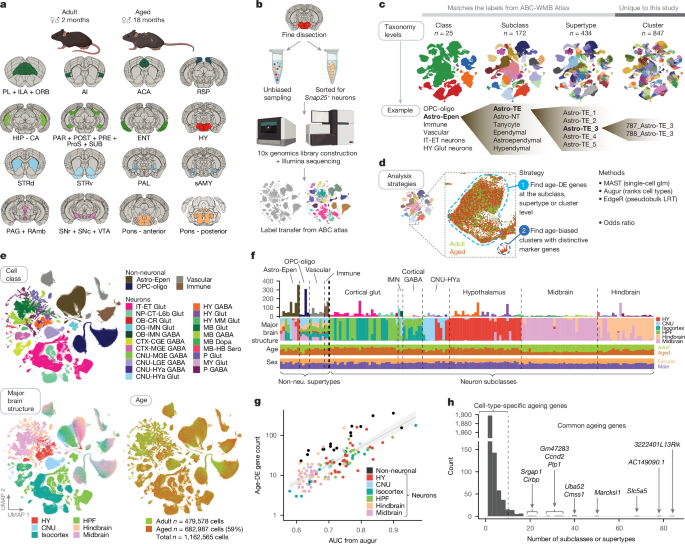
Off-target cell types were also collected because of dissection variability, and if included in the analysis, may result in bias of age analysis if certain libraries contained more off-target cells than others. To identify and remove these cell types from downstream analysis, we performed the following. First, using all the scRNA-seq data from the ABC-WMB atlas, we calculated the number and proportion of cells in that supertype that originated from the 16 regions included in this ageing study (Fig. 1a) versus other regions. The downstream analysis of supertypes that have less than 30% of cells from the 16 regions and have fewer than 500 cells were not included. A list of these supertypes found in the ABC-WMB atlas that were excluded due to off-target concerns are listed in Supplementary Table 2. The regions that were not targeted in the study are mostly the thalamus, medulla and olfactory regions.
where age and sex are all categorical variable each with two levels, and gene detection (gc) and QC score (qc) are log transformed and then z-score normalized, and the tilde (~) means distributed as. We included both gene detection and QC score in each model to account for potential effects that various FACS population plans had on library quality (Extended Data Fig. 6e,f The model with and without the age term had to be tested to generate P values. These P values were corrected for multiple hypothesis testing with the Bonferroni correction. The log2FC of the genes can be used to estimate the age effect size in the main body of the text.
Calculation and Analysis of the Global Molecular Plane Approximation (UMAP) from Principal Components Calculated from PCA
The UMAPs are calculated from the principal components calculated from PCA. For more than 100,000 cells, we used the imputed expression matrix of genes based on the top marker genes from each group of cells to perform PCA. No imputation was done for UMAPs with less than 100,000 cells. The number of principal components used to calculate projections, the amount of the local neighbourhood of cells and the size of the data can all be adjusted when generating UMAPs. For all UMAPs, the top 150 principal components were then selected, and principal components with more than 0.7 correlation with the technical bias vector (defined as log2(gene count) for each cell) were removed. Each UMAP was run with a set of different parameters, while each PCA had a different set of parameters. The global UMAP was calculated using the parameters of 988 genes, nn.neighbours, and 20 md.
The log2OR value for non-neuronal clusters are summarized in a diagram. 2b. Positive log2OR indicate clusters that are more biased towards aged cells than expected by chance (that is, age-enriched), whereas negative log2OR indicated clusters that are more biased towards young adult cells than expected by chance (that is, age-depleted). We highlight clusters with abs(log2OR) > 2.5.
All in situ spatial RNA data shown here were generated by Resolve Biosciences with their commercially available Molecular Cartography platform. Four total Molecular Cartography experiments were performed (RSTE1–4), each with a different panel of 100 genes and targeting different region(s) of the brain (Extended Data Fig. 5). For RSTE1, four different regions of the brain (cortex, striatum, midbrain and hindbrain) were imaged in both sexes and both ages (2 and 18 months), with two replicate brains per condition and two technical replicates per brain. The technical replicates were plotted and analysed as independent replicates in all figures. In RSTE2 the RSP and hippocampus were imaged, with four brains per condition. For RSTE3 and RSTE4, the hypothalamus was imaged in both sexes and both ages, with four replicate brains per condition. Brain samples were stored at 80 C for a few days and then shipped to San Jose, where the Molecular Cartography experiments were performed. After receipt of tissue, spot data was made available. Data analysis was performed at the Allen Institute using methods detailed below. Correlating transcript data was done using quality metrics that were generated from segmenting and mapping, and visualization was performed.
The fresh-frozen adult and aged brains were sectioned at 10 µm on Leica 3050 S cryostats. The OCT block containing a fresh-frozen brain was trimmed in the cryostat until reaching the desired region of interest. Sections were placed onto coverslips provided by Resolve Biosciences. Two replicate sections were collected sequentially: one as the primary sample and the other as a backup.
Cells were separated using a combination of open-source software. Cellpose uses a generalist algorithm for segmenting cells from images of cellular stains as input. Baysor uses a transcript-driven algorithm to draw cell boundaries based on transcript data alone while also having the option of integrating previous knowledge from stained images into the process. First, images of DAPI stains from each of the tissue samples were used as input for Cellpose using the following parameters: –pretrained_model = nuclei, –diameter = 0. The output of Cellpose was saved as a TIF file and used as a prior for the Baysor segmentation algorithm. The following input parameters were used to run Baysor.
To remove low-quality cells, we used a stringent QC process. Cells were first filtered by a broad set of quality cut-offs based on gene detection, QC score and doublet score. As we previously described3, the QC score was calculated by summing the log-transformed expression of a set of genes, whose expression level is decreased significantly in poor-quality cells. Briefly, these are housekeeping genes that are strongly expressed in nearly all cells with a very tight coexpression pattern that is anticorrelated with the nucleus-enriched transcript Malat1. We use this QC score to quantify the integrity of cytoplasmic messenger RNA (mRNA) content. Doublets were identified using a modified version of the DoubletFinder algorithm89. The cells included in this preliminary round of filtering had a gene detection greater than 1,000, a QC score greater than 50 and a doublet score less than 0.2. More than 1 million cells remained in the dataset using these thresholds. The table shows the mix of cell types by library and other categories.
The Reagent Kit v.3 was used for 10xv3 processing. We followed the manufacturer’s instructions for cell capture, barcoding, reverse transcription, complementary DNA amplification and library construction. We targeted a sequencing depth of 120,000 reads per cell; the actual average achieved was 77,743 ± 36,025 (mean ± s.d.) reads per cell across 287 libraries (Supplementary Table 1).
To enrich for neurons or live cells, cells were collected by FACS (BD FACSAria II or FACSAria Fusion, with FACSDiva v.8 software) using a 130 μm nozzle. Cells were prepared for sorting by passing the suspension through a 70 µm filter and adding Hoechst or 4,6-diamidino-2-phenylindole (DAPI) (to a final concentration of 2 ng ml−1). The sorting strategy was as previously described3,20, with most cells collected using the tdTomato-positive label. Then, 30,000 cells were sorted within 10 min into a tube containing 500 µl of quenching buffer. We found that sorting more cells into one tube diluted the ACSF in the collection buffer, causing cell death. We also observed decreased cell viability for longer sorts. Each 30,000 cells was gently layers on top of a 200 l BSA buffer and then centrifuged at 230g for ten minutes, with the high buffer at the bottom of the tube slowing down the cells as they reach it. The cells were resuspended after 35 l of buffer was removed and there was no pellet to be seen. Immediate centrifugation and resuspension allowed the cells to be temporarily stored in a high BSA buffer with minimal ACSF dilution. The resuspended cells were stored at 4 °C until all samples were collected, usually within 30 min. Samples from the same ROI were pooled, cell concentration quantified and immediately loaded onto the 10x Genomics Chromium controller.
Dissected tissue pieces were digested with 30 U ml−1 papain (Worthington, catalogue no. PAP2) in ACSF for 30 min at 30 °C. Owing to the short incubation period in a dry oven, we set the oven temperature to 35 °C to compensate for the indirect heat exchange, with a target solution temperature of 30 °C. Enzymatic digestion was quenched by exchanging the papain solution three times with quenching buffer (ACSF with 1% fetal bovine serum and 0.2% bovine serum albumin (BSA)). After 5 min, the samples were ready for trituration. The tissue pieces in the quenching buffer were triturated through a fire-polished pipette with a 600 µm diameter opening roughly 20 times. The tissue pieces were allowed to settle and the supernatant, which now contained suspended single cells, was transferred to a new tube. Fresh quenching buffer was added to the settled tissue pieces, and trituration and supernatant transfer were repeated using 300 and 150 µm fire-polished pipettes. The single-cell suspension was passed through a 70 µm filter into a 15 ml conical tube with 500 µl of high BSA buffer (ACSF with 1% fetal bovine serum and 1% BSA) at the bottom to help cushion the cells during centrifugation at 100g in a swinging bucket centrifuge for 10 min. The supernatant was discarded, and the cell pellet was resuspended in the quenching buffer. We collected 1,508,284 cells without performing FACS. The cells were loaded onto the 10X Genomics controller after the concentration of the resuspended cells was quantified.
Single cells were isolated by changing procedures. The brain was dissected, submerged in artificial cerebrospinal fluid (ACSF), embedded in 2% agarose and sliced into 350-μm coronal sections on a compresstome (Precisionary Instruments). Block-face images were captured during slicing. They were dissected from the slices and put into single cells. Fluorescent images of each slice before and after ROI dissection were taken at the dissection microscope. The images were used to show the exact location of the ROI.
All procedures were carried out in accordance with Institutional Animal Care and Use Committee protocols at the Allen Institute for Brain Science. Mice were provided food and water ad libitum and were maintained on a regular 14/10 h day/night cycle at no more than five adult animals of the same sex per cage. Ambient temperature of the vivarium was maintained between 21.1 and 22.78 °C (70–73 °F) and humidity was maintained between 40 and 45%. Mice were maintained on the C57BL/6J background. We excluded any mice with dermatitis, anophthalmia, microphthalmia, seizures or abdominal masses.
We used 44 aged mice (20 female, 24 male) and 64 young adult mice (31 female, 33 male) to collect cells for 10xv3 scRNA-seq. The young adult mice were included in the atlas. Young adult animals were euthanized at P 53–69 and older animals were euthanized at P540–553. No statistical methods were used to predetermine sample size. All donor animals used in this study are listed in Supplementary Table 1. The time of darkness and light within a 3h window was the same for all the tissue collections. We did not keep track of the oestrous cycle for female mice.
We isolated a total of 287 libraries from 108 animals: each animal contributed 1–6 libraries. Supplementary Table 1 has all the libraries listed. Transgenic driver lines were used for fluorescence-positive cell isolation by FACS to enrich for neurons. Roughly half the libraries (n = 145) were sorted for neurons from the pan-neuronal Snap25-IRES2-Cre line (JAX strain no. 023525) The Ai14-Tomatotd reporter is a JAX strain, and crossed to it. Supplementary Table 1. We used a variety of mice, including a few wild-type C57BL/6J mice. Unbiased sampling methods include libraries stained and sorted for Hoechst+, Calcein+/Hoechst+ or unstained libraries that were not sorted at all (no FACS). No FACS cells make up roughly 25% of the final high-quality dataset. The transgenic Snap25-IRES2-Cre line was backcrossed to C57BL/6J for at least ten generations before crossing and can be considered congenic. The transgenic Ai14 line was backcrossed to C57BL/6J for at least five generations before crossing and can be considered incipient congenic. Here are examples of gating strategies used for FACS.
We used the CCFv3 (RRID: SCR_002978) ontology22 (http://atlas.brain-map.org/) to define brain regions for profiling and boundaries for dissection. We covered the areas of the brain we thought were useful by sampling at the top-ontology level. The decisions were made because microdissections of small regions are difficult. Joint dissection of neighboring regions was necessary to get sufficient numbers of cells for profiling.